Install LightGBM and CatBoost on Ubuntu 22.04

Introduction

Working with machine learning is an interesting but lengthy journey. Most people start by picking up some fundamental concepts and then try to apply them using straightforward methods. One of the first approaches we encounter — whether in learning guides or at university — is logistic and linear regression. These are techniques that are easy to understand in terms of how they work, and they offer an acceptable level of accuracy. When it comes to prediction problems, however, there are now strong alternatives with higher predictive power. One of them is Gradient Boosting Machines (GBMs), which substantially improve our model’s predictions without being particularly demanding to use.

Before we can use them — for example through the tidymodels package — we need to install the corresponding software. In this article we summarise the installation instructions for each one.

Table 1: Boosting algorithms and their documentation pages

Model	Documentation
LightGBM	Link
CatBoost	Link
XGBoost	Link

library(highcharter)
library(gtrendsR)
library(dplyr)

googleTrendsData <- gtrendsR::gtrends(
  keyword      = c("LightGBM", "CatBoost", "XGBoost"),
  gprop        = "web",
  onlyInterest = TRUE
)

interestOverTime <- googleTrendsData[["interest_over_time"]] %>%
  dplyr::mutate(date = lubridate::ymd(date)) %>%
  dplyr::mutate(Year = lubridate::year(date)) %>%
  select(Year, keyword, hits) %>%
  group_by(Year, keyword) %>%
  summarise(Average = round(mean(hits), digits = 1), .groups = "drop")

highchart() %>%
  hc_chart(type = "line") %>%
  hc_title(text = "Search engine interest over time") %>%
  hc_subtitle(text = "Comparing search trends across Gradient Boosting Machine algorithms (GBMs).") %>%
  hc_xAxis(categories = unique(interestOverTime$Year)) %>%
  hc_yAxis(title = list(text = "Trend")) %>%
  hc_add_series(
    name = "XGBoost",
    data = interestOverTime %>% filter(keyword == "XGBoost") %>% pull(Average)
  ) %>%
  hc_add_series(
    name = "CatBoost",
    data = interestOverTime %>% filter(keyword == "CatBoost") %>% pull(Average)
  ) %>%
  hc_add_series(
    name = "LightGBM",
    data = interestOverTime %>% filter(keyword == "LightGBM") %>% pull(Average)
  )

LightGBM

LightGBM was developed by Microsoft and released in 2016. Its main advantage is speed and low memory consumption. This makes it an ideal choice when working with very large datasets, where other implementations may become slow or exhaust the available memory.

Option 1 — Installing the R package

The simplest way to install LightGBM for R users is through the corresponding lightgbm package, directly from CRAN:

elapsed_lightgbm <- system.time(
  install.packages("lightgbm", repos = "https://cran.r-project.org")
)[["elapsed"]]

Option 2 — Installing via CMake

If we prefer to build from source, the LightGBM documentation page covers the process in detail. The basic commands for Linux are as follows:

Terminal

sudo apt install cmake

Terminal

git clone --recursive https://github.com/microsoft/LightGBM
cd LightGBM
mkdir build
cd build
cmake ..
make -j4

CatBoost

CatBoost was developed by Yandex and released in 2017. It differs from the other implementations mainly in how it handles categorical features: whereas these typically require preprocessing (e.g. one-hot encoding), CatBoost can work with them directly, without any transformation. This makes it particularly useful for datasets with many categorical variables, as is often the case in commercial and financial applications. It also tends to require less hyperparameter fine-tuning compared to the alternatives.

CatBoost is not available on CRAN, so we use the install_url() function from devtools, passing a link from the official releases page on GitHub.

Warning

When installing devtools, an error may appear due to the missing system libraries libharfbuzz-dev and libfribidi-dev. If we encounter this issue (which is common on Ubuntu 22), installing them and restarting RStudio is enough to resolve it:

Terminal

sudo apt install libharfbuzz-dev libfribidi-dev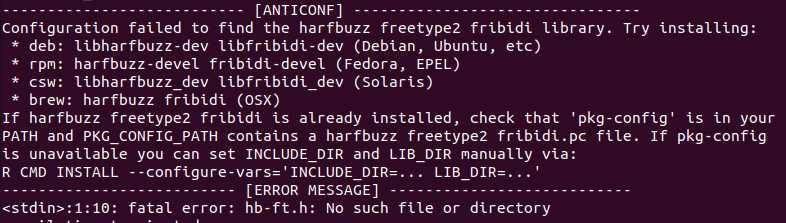

Error message when installing devtools

elapsed_catboost <- system.time(
  devtools::install_url(
    "https://github.com/catboost/catboost/releases/download/v1.1.1/catboost-R-Linux-1.1.1.tgz",
    INSTALL_opts = c("--no-multiarch", "--no-test-load")
  )
)[["elapsed"]]

XGBoost

XGBoost (Extreme Gradient Boosting) was developed by Tianqi Chen and introduced in 2016. It is historically the most widely adopted GBM implementation: it won dozens of Kaggle competitions and became almost synonymous with the term “gradient boosting” for several years. It consistently outperforms classical methods (logistic/linear regression, Naive Bayes, etc.) and offers a rich set of hyperparameter tuning options. It is worth noting that on very large datasets it may fall behind LightGBM in terms of speed.

Installation is just as straightforward as with lightgbm:

elapsed_xgboost <- system.time(
  install.packages("xgboost")
)[["elapsed"]]

Summary

Gradient Boosting Machines offer higher predictive power compared to classical machine learning methods, and installing them in R is a relatively straightforward process.

As a small experiment, we timed the installation of each package using the system.time() function. The results are summarised in the table below:

Note

The times were measured on a specific system and network connection. They may vary depending on hardware, R version, and internet speed.

Table 2: Installation times for common Gradient Boosting algorithms

Model	Installation method	Installation time
LightGBM	R package	7.79 minutes
CatBoost	Release link	2.1 minutes
XGBoost	R package	6.16 minutes