Introduction
And here we go…
This is the first notebook on my website and I’d like to be a little special. I didn’t want to just take a ready-made dataset and apply a machine learning technique (I will do this in the next articles). So, I decided to make my own with the help of hellenic’s parliament website.
The Greek political scene has particularly preoccupied global public opinion in recent years, due to the Greek economic crisis. A part of it was spent on the reasons that caused it. The causes of the Greek crisis are many and a point of contention to this day. In this article we will deal essentially with one of the points of criticism. The election of the same persons.
With this notebook I will try to analyze whether this claim is valid by counting how many times someone has been elected to the Greek parliament. In addition, I will study the obsession with the same persons at the party level, but also at the local level (constituencies).
Prerequisites
Import Libraries
First and foremost, we have to load our libraries.
Import dataset
After loading R libraries, then I will load my data.
Show the code
parliament <- read_csv("data/greek_parliament.csv")Preview Dataset
Show the code
preview_dataset = head(parliament, 10)
kbl(preview_dataset,
    align = 'c',
    booktabs = T,
    centering = T,
    valign = T) %>%
  kable_paper() %>%
scroll_box(width = "600px", height = "250px")| FullName | Party | Constituency | Term |
|---|---|---|---|
| Agorastis Vasileios | PA.SO.K. (Panhellenic Socialist Movement) | Larissa | 3 |
| Akrita Sylva - Kaiti | PA.SO.K. (Panhellenic Socialist Movement) | Athens B | 3 |
| Akritidis Nikolaos | PA.SO.K. (Panhellenic Socialist Movement) | Thessaloniki A | 3 |
| Akrivakis Alexandros | PA.SO.K. (Panhellenic Socialist Movement) | Viotia | 3 |
| Alevras Ioannis | PA.SO.K. (Panhellenic Socialist Movement) | Athens A | 3 |
| Alexandris Efstathios (Stathis) | PA.SO.K. (Panhellenic Socialist Movement) | Athens B | 3 |
| Alexiadis Konstantinos | PA.SO.K. (Panhellenic Socialist Movement) | Trikala | 3 |
| Alexiou Thomas | NEA DIMOKRATIA | Xanthi | 3 |
| Allamanis Stylianos | NEA DIMOKRATIA | Karditsa | 3 |
| Amanatidis Konstantinos | PA.SO.K. (Panhellenic Socialist Movement) | Thessaloniki B | 3 |
Structure of Dataset
| Variable | Property | Description |
|---|---|---|
Full Name |
qualitative (nominal) |
Surname and name of the member of parliament |
Party |
qualitative (nominal) |
The party on which the MP got elected |
Constituency |
qualitative (nominal) |
MP got elected on this area |
Term |
qualitative (ordinal) |
Plenum term |
Thus, my sample has 4 variables, of which 0 are quantitative and 4 are quantitative properties, of which 3 are nominal and the rest one (Term) is ordinal.
Recoding variables
Party names can vary from short to lengthy ones. The last ones are a problem for our analysis because their names can not fit to our visualisations. The table below is showing all the parties that have ever participated in parliament. Is is apparent that some parties have really long names.
Show the code
data.frame(
  Party = unique(parliament$Party),
  Length = str_length(unique(parliament$Party))
) %>%
  arrange(-Length) %>%
  reactable(
    defaultPageSize = 5
  )
In our case the parties with the longest name is AN.EL. and Democratic Coalition with 81 and 70 characters, respectively. On the contrary, the shortest party name is POL.A. with 6 characters.
Show the code
## Recoding parliament$Party
parliament$Party[parliament$Party == "ANEXARTITOI DIMOKRATIKOI VOULEFTES"] <- "ADP"
parliament$Party[parliament$Party == "ANEXARTITOI ELLINES (Independent Hellenes)"] <- "ANEL"
parliament$Party[parliament$Party == "ANEXARTITOI ELLINES (Independent Hellenes) National Patriotic Democratic Alliance"]<- "ANEL"
parliament$Party[parliament$Party == "Coalition of the Left and Progress"] <- "SYRIZA"
parliament$Party[parliament$Party == "Communist Party of Greece (Interior)"] <- "KKE (interior)"
parliament$Party[parliament$Party == "DEMOCRATIC COALITION (Panhellenic Socialist Movement Democratic Left )"] <- "PASOK"
parliament$Party[parliament$Party == "DHM.AR (Democratic Left)"] <- "DHMAR"
parliament$Party[parliament$Party == "DI.ANA."] <- "DIANA"
parliament$Party[parliament$Party == "DI.K.KI."] <- "DIKKI"
parliament$Party[parliament$Party == "INDEPENDENT"] <- "INDEPENDENT"
parliament$Party[parliament$Party == "KOMMOUNISTIKO KOMMA ELLADAS"] <- "KKE"
parliament$Party[parliament$Party == "LA.O.S."] <- "LAOS"
parliament$Party[parliament$Party == "LAIKI ENOTITA"] <- "LAE"
parliament$Party[parliament$Party == "LAIKOS SYNDESMOS - CHRYSI AVGI (People’s Association – Golden Dawn)"] <- "XA"
parliament$Party[parliament$Party == "NEA DIMOKRATIA"] <- "ND"
parliament$Party[parliament$Party == "PA.SO.K. (Panhellenic Socialist Movement)"] <- "PASOK"
parliament$Party[parliament$Party == "POL.A."] <- "POLA"
parliament$Party[parliament$Party == "SYNASPISMOS RIZOSPASTIKIS ARISTERAS"] <- "SYRIZA"
parliament$Party[parliament$Party == "TO POTAMI (The River)"] <- "POTAMI"
parliament$Party[parliament$Party == "ΟΟ.ΕΟ."] <- "EO"
Setting colors
A few days after, I decided that there should be a consistency in the choice of colors. That’s the reason of this section. Thus, I will assign a dedicated hex color code to each party.
Show the code
parties = data.frame(
  Party = unique(parliament$Party)
) |>
  mutate(Color = case_when(
    Party == "PASOK" ~ "#95bb72",
    Party == "ND" ~ "#0492c2",
    Party == "KKE" ~ "#FF6666",
    Party == "SYRIZA" ~ "#e27bb1",
    Party == "KKE (interior)" ~ "#FF3366",
    Party == "INDEPENDENT" ~ "#ffffff",
    Party == "DIANA" ~ "orange",
    TRUE ~ "#808080"
  ))

kke_color = "#FF6666"
nd_color = "#0492c2"
pasok_color = "#95bb72"
syriza_color = "#e27bb1"
Show the code
names = c("Panhellenic Socialistic Mpvement", "New Democracy", "Communist Party of Greece", "Communist Party οf Greece (interior)",
          "Independent", "Coalition of the Radical Left", "Democratic Renewal", "Alternative Ecologists", "Political Spring",
          "Democratic Social Movement", "Popular Orthodox Rally", "Democratic Left", "Independent Greeks", "Golden Dawn", "Independent Democratic MPs",
          "Popular Unity", "The River")

parties$names = names

parties$Party_el= c("ΠΑΣΟΚ", "ΝΔ", "ΚΚΕ", "ΚΚΕ (εσωτερικού)", "Ανεξάρτητοι", "ΣΥΡΙΖΑ", "ΔΗΑΝΑ", "ΕΟ", "ΠΟΛΑΝ", "ΔΗΚΚΙ",
             "ΛΑΟΣ", "ΔΗΜΑΡ", "ΑΝΕΛ", "ΧΑ", "ΑΔΒ", "ΛΑΕ", "ΠΟΤΑΜΙ")

parties$names_el = c("Πανελλήνιο Σοσιαλιστικό Κίνημα", "Νέα Δημοκρατία", "Κομμουνιστικό Κόμμα Ελλάδας",
                    "ΚΚΕ (εσωτερικού)","Ανεξάρτητοι", "Συνασπισμός Ριζοσπαστικής Αριστεράς", "Δημοκρατική Ανανέωση",
                    "Εναλλακτικοί Οικολόγοι", "Πολιτική Άνοιξη",
            "Δημοκρατικό Κοινωννικό Κίνημα", "Λαϊκός Ορθόδοξος Συναγερμός", "Δημοκρατική Αριστερά", "Ανεξάρτητοι Έλληνες",
            "Χρυσή Αυγή", "Ανεξ Δημ. Βουλευτές", "Λαϊκή Ενότητα", "Το Ποτάμι")
Parliament over the years
Now, I will make a short sum-up of the electoral resuts over the years. It is important to share that I made it thanks to this post and ggpol package. As I am planning to do this procedure for many electoral terms, I will convert it as a function.
Arguments like term and custom_title are vital to create reproducible plots for all the terms. Although a main problem is the colors. On the aforementioned post it was about only one term. We knew how many parties we had, so we knew what colors to set and how many. If we try that on many terms (on which the number of parties can vary from 3 to 8) an error will come up which will say “Hey, you have set 3 colors but I see that you have 8 values (parties)”. This was a real obstacle for me. After some tries and misses I came up with the concept of dynamic arguments.
Show the code
make_parliament_plot <- function(term, custom_title, ...){

custom = parliament %>% filter(Term == term) %>% select(Party) %>% table() %>% t() %>% as.data.frame() %>%  `colnames<-`(c("","Party", "Seats"))

colors<-c(...)

custom$legend <- paste0(custom$Party," (", custom$Seats,")")

#draw a parliament diagram
p<-ggplot(custom) +
  geom_parliament(aes(seats =Seats, fill =  Party), color = "white") +
  scale_fill_manual(values = colors , labels = custom$legend) +
  coord_fixed() +
  theme_void()+
  labs(title  = custom_title,
       caption = "Source: stesiam | stesiam.github.io, 2022")+
  theme(title = element_text(size = 18),
        plot.title = element_text(hjust = 0.5,size = 14,face = 'bold'),
        plot.subtitle = element_text(hjust = 0.5),
        plot.caption = element_text(vjust = -3,hjust = 0.9, size = 8),
        legend.position = 'bottom',
        legend.direction = "horizontal",
        legend.spacing.y = unit(0.1,"cm"),
        legend.spacing.x = unit(0.1,"cm"),
        legend.key.size = unit(0.8, 'lines'),
        legend.text = element_text(margin = margin(r = 1, unit = 'cm')),
        legend.text.align = 0)+
        guides(fill=guide_legend(nrow=3,byrow=TRUE,reverse = TRUE,title=NULL))

return(p)
}
Show the code
# f1 = parliament %>%
#   dplyr::count(FullName, Party) %>%
#   arrange(-n) %>%
#   dplyr::filter(n>=9) %>%
#   mutate(lastName = extract_name_parts_vec(FullName))
#
# party_colors = c(
# kke_color = "#FF6666",
# nd_color = "#0492c2",
# pasok_color = "#95bb72",
# syriza_color = "#e27bb1")
#
# points <- purrr::pmap(
#   list(
#     y = f1$n,
#     color = party_colors[f1$Party]
#   ),
#   function(y, color) list(y = y, color = color)
# )

# highchart() %>%
#   hc_chart(type = "bar") %>%
#   hc_title(text = "Top 20 Politicians by Times Elected") %>%
#   hc_xAxis(
#     categories = f1$lastName$last_name,
#     title = list(text = "Politician")
#   ) %>%
#   hc_yAxis(title = list(text = "Times Elected")) %>%
#   hc_add_series(
#     data = points,
#     name = "Times Elected",
#     colorByPoint = TRUE,
#     showInLegend = FALSE
#   ) %>%
#   hc_tooltip(pointFormat = "<b>{point.category}</b><br>Times elected: {point.y}")
Note that till this moment I have not figure out how to change the position of the parties in an efficient way (in a function) that will somehow represent their potitical view. The next visualizations of the parliament are exclusively about how many MPs got elected by each party.
Show the code
plot_parliament_term <- function(term_num, parliament_data, parties_data, lang = "en") {
  # Filter the parliament data for the selected term and summarize by party
  term_data <- parliament_data |>
    dplyr::filter(Term == term_num) |>
    group_by(Party) |>
    summarise(n = n()) |>
    ungroup()

  # Perform fuzzy join with parties data based on party name similarity
  term_data_joined <- fuzzyjoin::stringdist_inner_join(term_data, parties_data, by = "Party",
                                                      max_dist = 2, distance_col = "distance") |>
    group_by(Party.x) |>
    slice_min(distance) |>   # Ensure only the closest match is selected
    rename(Party = Party.x)

  # Conditionally adjust the data based on language
  if (lang == "en") {
    term_data_joined <- select(term_data_joined, names, Party, n, Color)
    title_text = "Distribution of seats"
    subtitle_text = "Final formation of Hellenic Parliament"
    caption_text = '<b>Source:</b> Hellenic Parliament | <b>Graphic:</b> <a href="https://stesiam.com/" target="_blank">stesiam.com</a>'
    hover_text = "Representatives"
  } else {
    term_data_joined <- select(term_data_joined, names_el, Party_el, n, Color)
    title_text = "Κατανομή θέσεων"
    subtitle_text = "Τελική μορφή Ελληνικού Κοινοβουλίου"
    caption_text = '<b>Πηγή:</b> Ελληνικό Κοινοβούλιο | <b>Γράφημα:</b> <a href="https://stesiam.com/" target="_blank">stesiam.com</a> '
    hover_text = "Βουλευτές"
  }

  # Create the highcharter plot for the specific term
  highchart() %>%
    hc_chart(type = 'item') %>%
    hc_title(text = title_text) %>%
    hc_subtitle(text = subtitle_text) %>%
    hc_caption(
      text = caption_text,
      align = 'center',
      verticalAlign = 'bottom',
      y = 10
    ) %>%
    hc_legend(labelFormat = '{name} <span style="opacity: 0.4">{y}</span>') %>%
    hc_add_series(
      name = hover_text,
      data = purrr::pmap(
        if (lang == "en") {
          list(term_data_joined$names, term_data_joined$n, term_data_joined$Color, term_data_joined$Party)
        } else {
          list(term_data_joined$names_el, term_data_joined$n, term_data_joined$Color, term_data_joined$Party_el)
        },
        list
      ),
      keys = c("name", "y", "color", "label"),
      dataLabels = list(
        enabled = TRUE,
        format = "{point.label}",
        style = list(textOutline = "5px contrast")
      ),
      center = list("50%", "88%"),
      size = "170%",
      startAngle = -100,
      endAngle = 100
    ) %>%
 hc_responsive(
  rules = list(
    list(
      condition = list(maxWidth = 600),
      chartOptions = list(
        series = list(
          dataLabels = list(
            distance = -30,
            style = list(
              fontSize = "12px",
              textOutline = "1px contrast"  # Outline for labels
            )
          ),
          center = list("50%", "75%"),  # Adjust center position for mobile
          size = "130%"
        )
      )
    ),
    list(  # New condition for max width of 400px
      condition = list(maxWidth = 400),
      chartOptions = list(
        series = list(
          dataLabels = list(
            distance = -20,
            style = list(
              fontSize = "9px",        # Smaller font for smaller screens
              textOutline = "1px contrast"  # Maintain outline
            )
          ),
          center = list("50%", "80%"),  # Further adjust center position for even smaller screens
          size = "110%"   # Adjust the size for smaller screens
        )
      )
    )
  )
)
}
Show the code
plot_parliament_term(3,parliament, parties, lang = "en")Show the code
plot_parliament_term(4,parliament, parties, lang = "el")Adding missing grouping variables: `Party`Show the code
plot_parliament_term(5,parliament, parties)Show the code
plot_parliament_term(6,parliament, parties)Show the code
plot_parliament_term(7,parliament, parties)Show the code
plot_parliament_term(8,parliament, parties)Show the code
plot_parliament_term(9,parliament, parties, lang = "el")Adding missing grouping variables: `Party`Show the code
plot_parliament_term(10,parliament, parties)Show the code
plot_parliament_term(11,parliament, parties)Show the code
plot_parliament_term(12,parliament, parties)Show the code
plot_parliament_term(13,parliament, parties)Show the code
plot_parliament_term(14,parliament, parties)Show the code
plot_parliament_term(15,parliament, parties)Show the code
plot_parliament_term(16,parliament, parties)As you can see on the next plot there are many MPs that are classified as independent (according to Hellenic’s Parliament website). Many of them are members of parties “ANEL” and “Enosi Kentroon”. However, a large wave of departures from the parties led to not fulfilling the conditions to be considered as parliamentary parties. For that reason members of these parties (that did not left) are considered independent.
Show the code
plot_parliament_term(17,parliament, parties)Most elected members of parliament
Show the code
#total_times_elected_freqs <- function(input_constituency, min_times_elected){
total_times_elected_freqs_df = parliament %>%  count(FullName, Party) %>% filter(n >= 9) %>% as.data.frame()

#df = table(parliament$FullName)%>% sort(decreasing = T) %>% as.data.frame() %>% filter(Freq>=11)

ggplot(data = total_times_elected_freqs_df, aes(x = reorder(FullName, n), y = n, fill = Party ))+
  geom_bar(stat = "identity",width = 0.88) +
  geom_text(aes(label=n), hjust = 1.5, vjust=0.5, color="white", size=4)+
  theme_minimal() +
  scale_fill_manual(values = c("KKE" = kke_color,"ND" = nd_color, "PASOK" = pasok_color, "SYRIZA" = syriza_color)) +
  labs(title = "Most elected MPs on Greek Parliament (1981 - 2019) <br>
       <span style = 'font-size:10pt'> A list that shows the most elected members of parliament (elected 11 times or more). <br> The following ones are members of <span style = 'color:blue;'>ND</span>,  or <span style = 'color:darkgreen;'>PASOK</span></span>.",
       caption = "Source: **stesiam** | stesiam.github.io, 2022",
       x = "Times elected",
       y = "Members of Parliament") +
    theme(
    plot.title.position = "plot",
    plot.title = element_textbox_simple(
      size = 14,
      lineheight = 1,
      padding = margin(5.5, 5.5, 5.5, 5.5),
      margin = margin(0, 0, 5.5, 0),
      fill = "cornsilk"
    ))+
  coord_flip()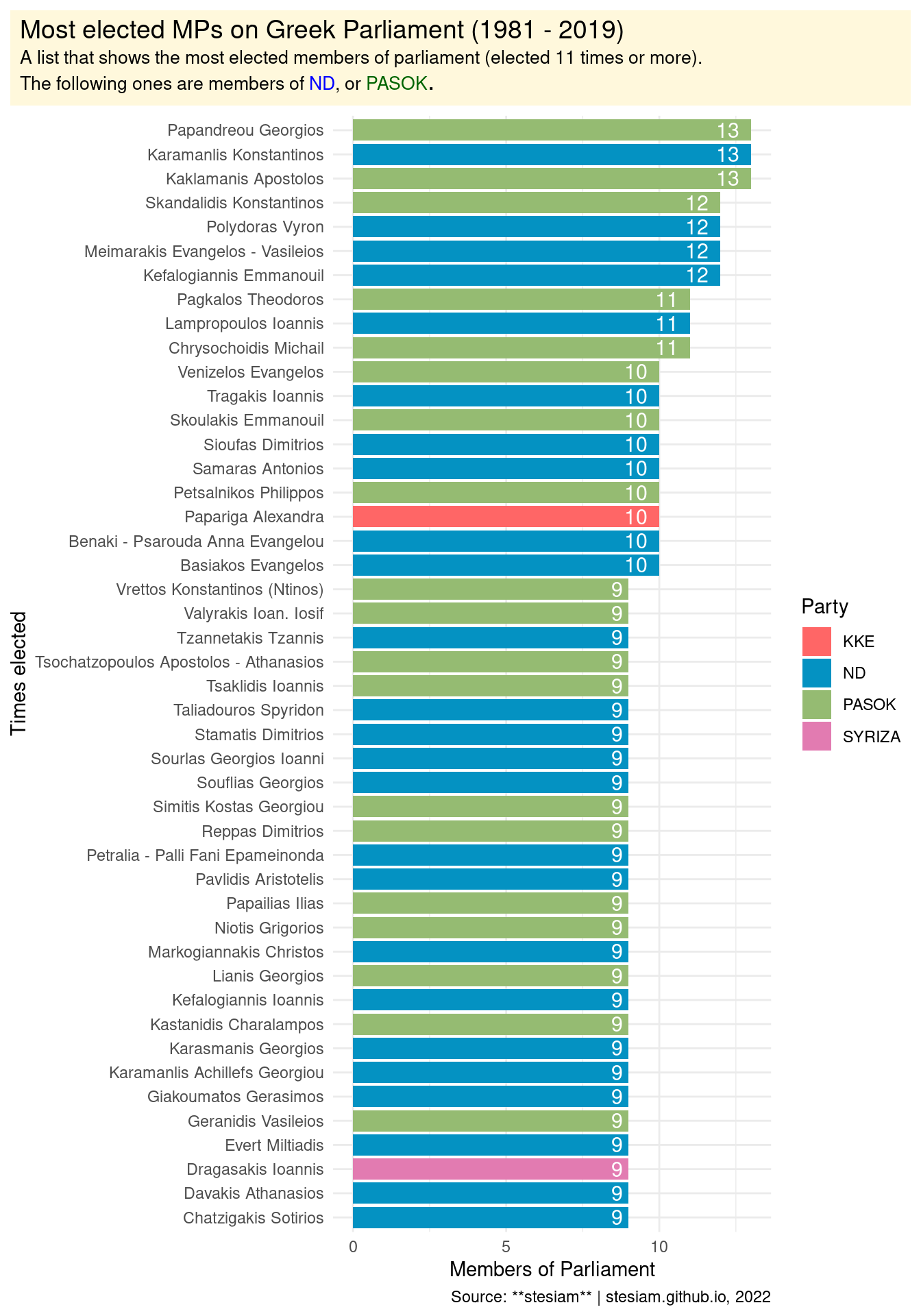
Most elected members by party
So far we have seen the most elected members of Greek parliament for the period 1981-2019. Ιt would be particularly interesting to study the same feature by party. However, finding the most elected member per party can be challenging on parties with relatively low representation on Greek parliament. That is the reason for choosing only some of those.
Concerning the implementation part, I see that I will make some visualizations with minimum changes (e.g., filter dataset based on party, change color, etc.) so, the creation of a function is justified. That way, I will not repeat same code, following one of the principles of programming (DRY - Don’t Repeat Yourself). On the following function we can see that I set 3 variables :
-
Party: I have to specify which data to filter -
color: In order to customize color of my barplots to be similar to each party’s color -
times_elected_min: A argument that I added up later. The problem with its absence is that I have to deal with parties that elect for example 150 MPs and some others just 10. If I set a universal number of elections to visualize I will have diagrams with many problems. Let’s suppose that I set a big value (e.g., 10). Then I would visualize my data for ND and PASOK, although parties with relatively low number of MPs would have only one or noone to show (KKE & SYRIZA, respectively). On the other hand if I set a low value I create a new problem as there will be many MPs of and it creates the need to edit many more things (like width of bars). An argument liketimes_elected_mincan adapt the specific characteristics of each party.
Show the code
party_plot <- function(party, party_color, times_elected_min) {

  party_df <- parliament %>%
    dplyr::filter(Party == party) %>%
    count(FullName) %>%
    arrange(-n) %>%
    as.data.frame() %>%
    dplyr::filter(n >= times_elected_min)


highchart() %>%
    hc_chart(type = "bar", inverted = TRUE) %>%
    hc_title(text = glue("Most elected MPs of {party}")) %>%
    hc_subtitle(text = glue()) %>%
    hc_xAxis(
      categories = party_df$FullName,
      title = list(text = "Members of Parliament"),
      labels = list(
        style = list(fontSize = "11px", whiteSpace = "normal"),
        useHTML = TRUE
      )
    ) %>%
    hc_yAxis(title = list(text = "Times elected")) %>%
    hc_add_series(
      name = "Times elected",
      data = party_df$n,
      color = party_color
    ) %>%
    hc_plotOptions(bar = list(dataLabels = list(enabled = TRUE))) %>%
    hc_tooltip(pointFormat = "<b>{point.category}</b>: {point.y} times elected") %>%
    hc_legend(enabled = FALSE)  # Hides the legend
}
The visualizations are presented in alphabetical order.
KKE
Show the code
party_plot("KKE", "#FF6666", times_elected_min = 5)ND
Show the code
party_plot("ND", "#0492c2", times_elected_min = 10)PASOK
Show the code
party_plot("PASOK", "#95bb72", times_elected_min = 10)SYRIZA
Show the code
party_plot("SYRIZA", "#e27bb1", times_elected_min = 5)Most elected members based per constituency
So far we have seen :
- the composition of Greek Parliament
- the most elected MPs on national level and
- the most elected MPs on party level
The last part of my analysis will investigate the most popular MPs on local level (per profecture).
Obviously, the same logic applies to party charts (same processes with minor changes), so the use of a function is almost mandatory (over fifty -50- cases !).
On my previous workflow I used table() function in order to take frequencies. That’s one easy way to go. Although I didn’t figured out to add characteristics from other columns (like party of the MP). Fir that reason I took the decision to use count() instead of table.
Show the code
constituency_freqs <- function(input_constituency, min_times_elected){
cont_df = parliament %>% filter(Constituency == input_constituency) %>%
  count(FullName, Party) %>% filter(n >= min_times_elected) %>% as.data.frame()

  ggplot(data = cont_df, aes(x = reorder(FullName, n), y = n, fill = Party ))+
  geom_bar(stat = "identity",width = 0.88) +
  scale_fill_manual(values = c("ANEL" = "#bcd2e8", "INDEPENDENT" = "#cccccc","KKE"=kke_color,"ND" = nd_color, "PASOK" = pasok_color, "SYRIZA" = syriza_color,"XA" = "#000000")) +
  geom_text(aes(label=n), hjust = 1.5, vjust=0.5, color="white", size=4)+
  theme_minimal() +
   labs(title = "Most elected MPs",
       subtitle = "",
       caption = "Source: stesiam | stesiam.github.io, 2022") +
  coord_flip()
}
Now I have frequencies and the party for every MP. That will be useful on my diagrams.
Show the code
#unique(parliament$Constituency) %>% sort()State
Show the code
constituency_freqs("State", 3)
Attica
Show the code
constituency_freqs("Athens A",5)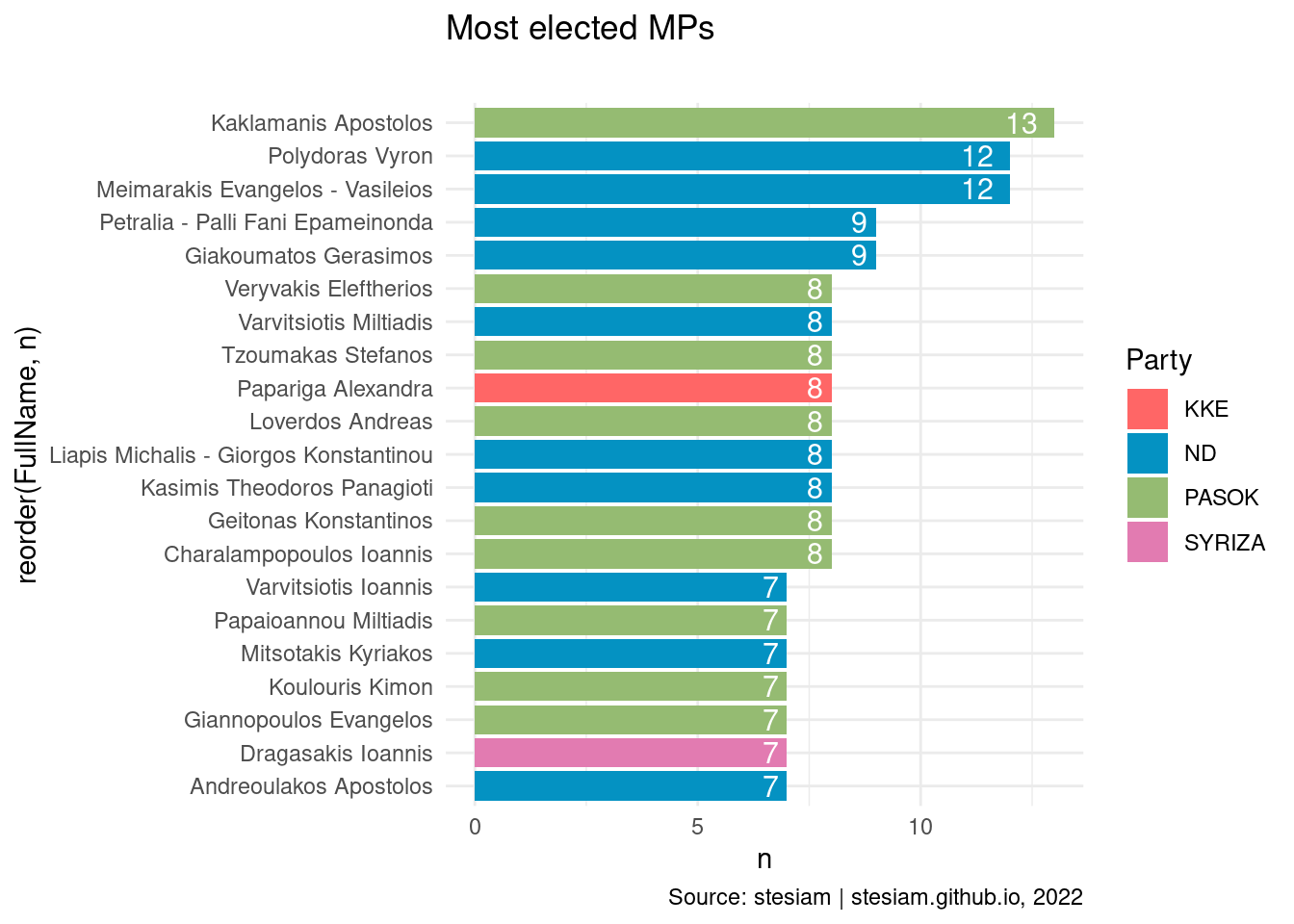
Show the code
constituency_freqs("Athens B",7)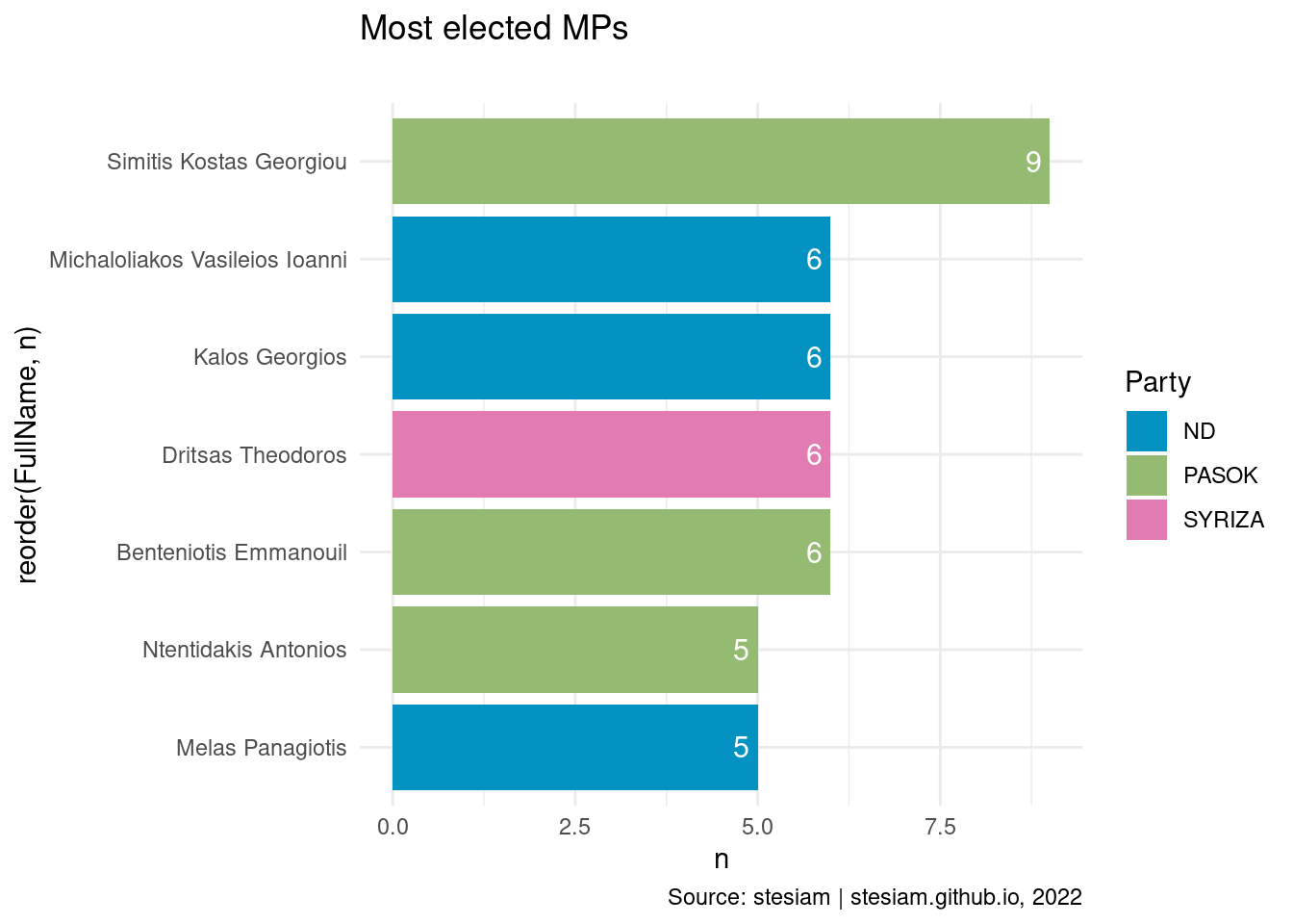
Show the code
constituency_freqs("Piraeus A",5)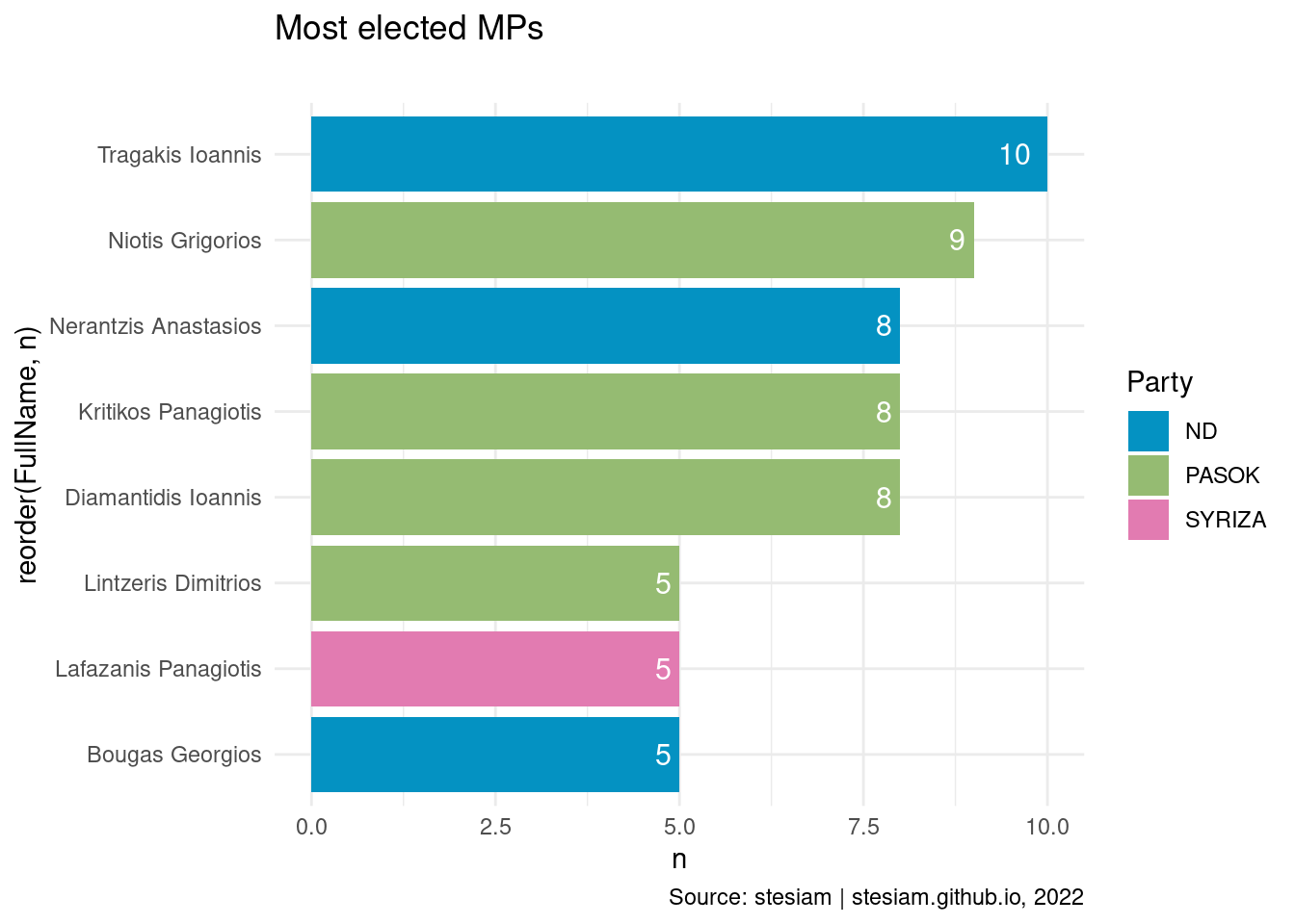
Show the code
constituency_freqs("Piraeus B",5)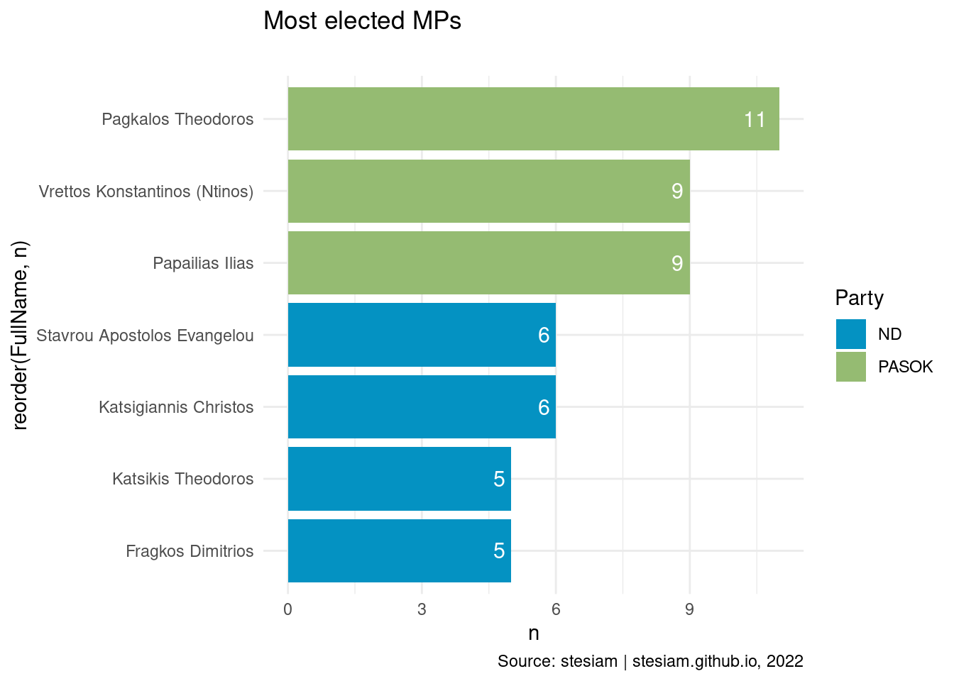
Show the code
constituency_freqs("Of Attica (rest)",5)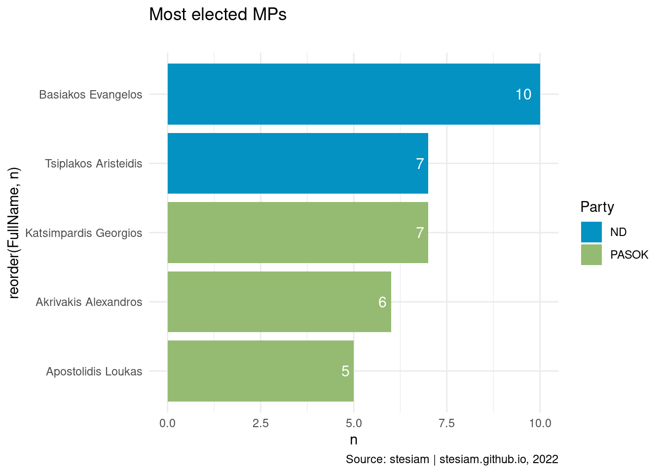
Central Greece
Show the code
constituency_freqs("Viotia",5)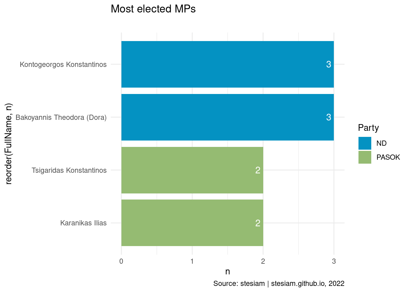
Show the code
constituency_freqs("Evrytania",2)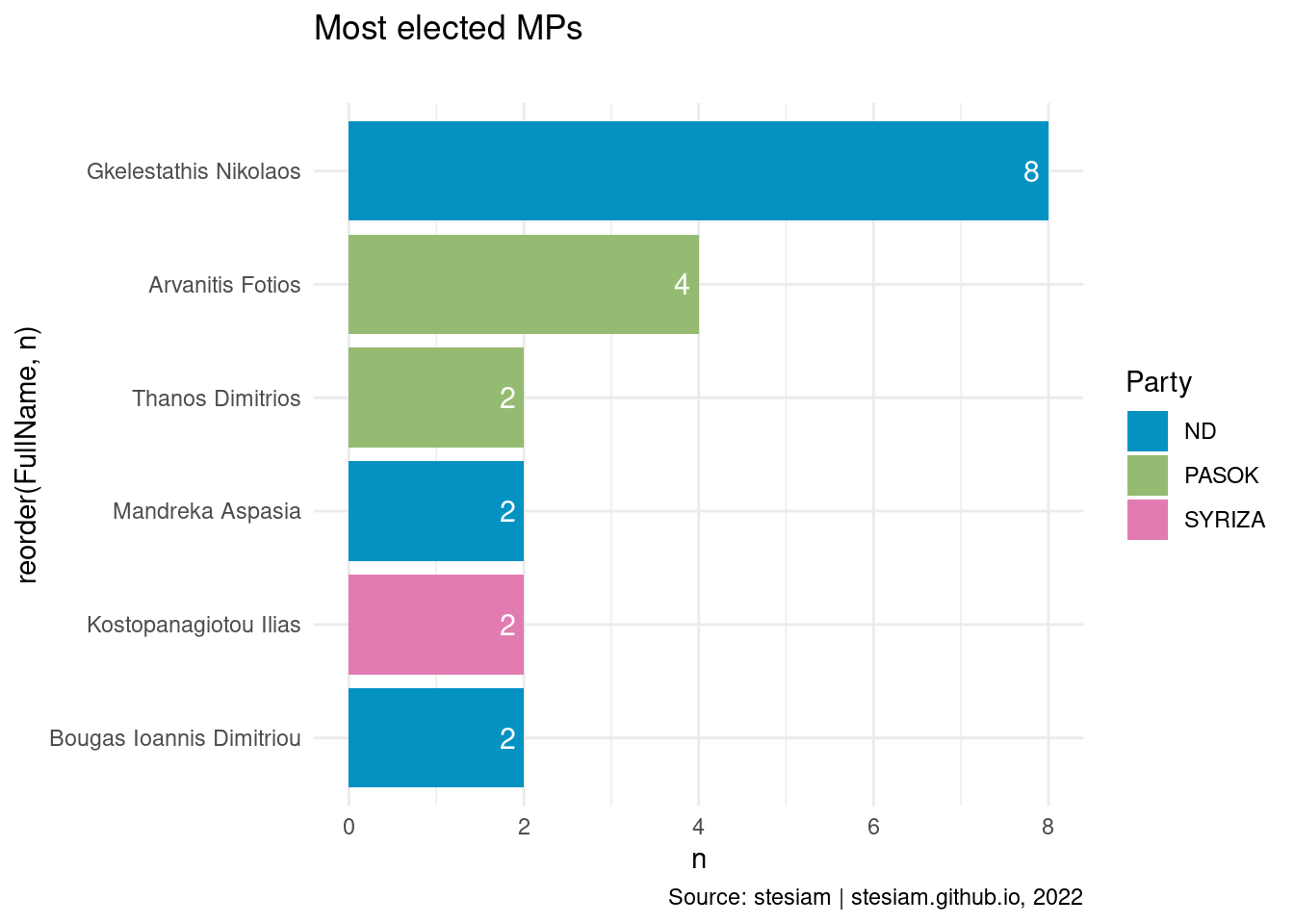
Show the code
constituency_freqs("Fokida",2)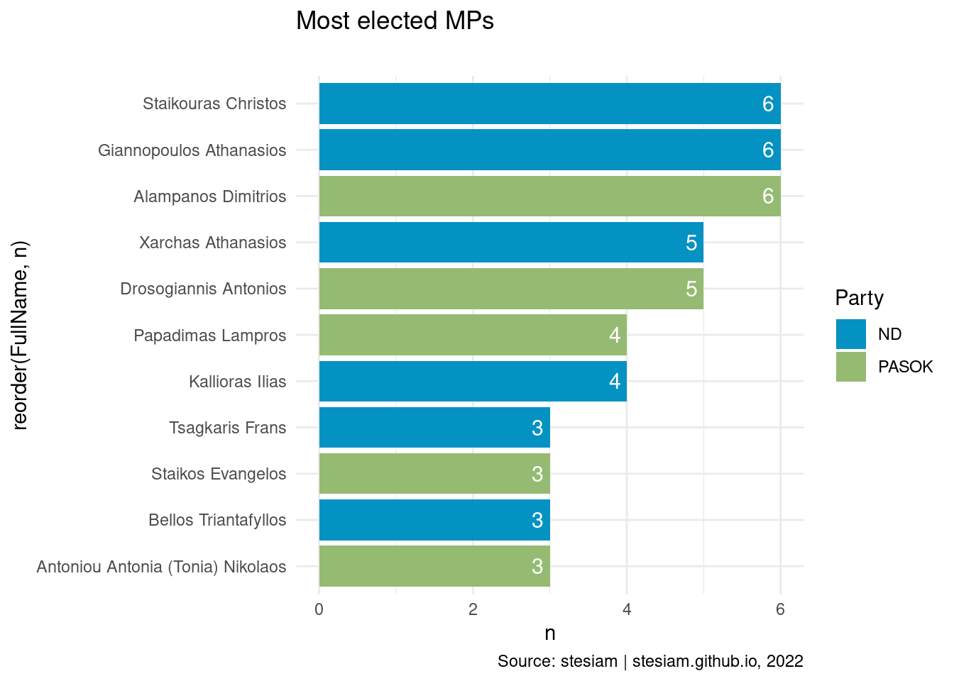
Show the code
constituency_freqs("Fthiotida",3)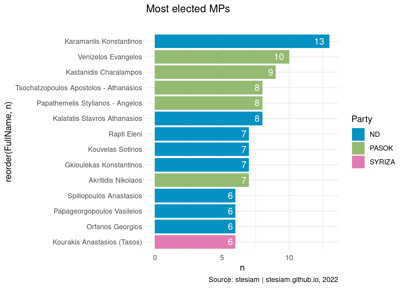
Central Macedonia
Show the code
constituency_freqs("Thessaloniki A",6)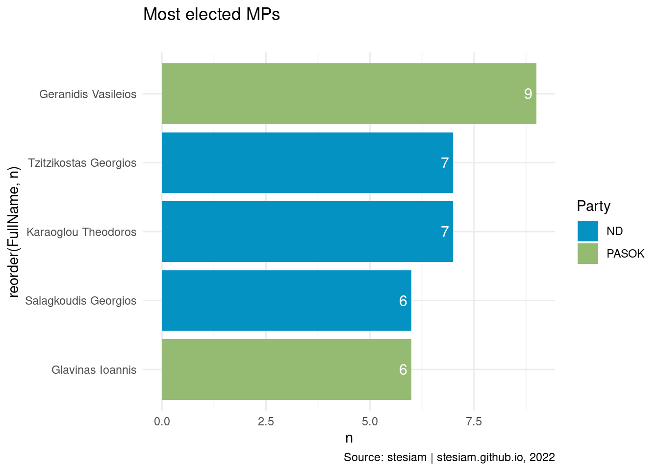
Show the code
constituency_freqs("Thessaloniki B",6)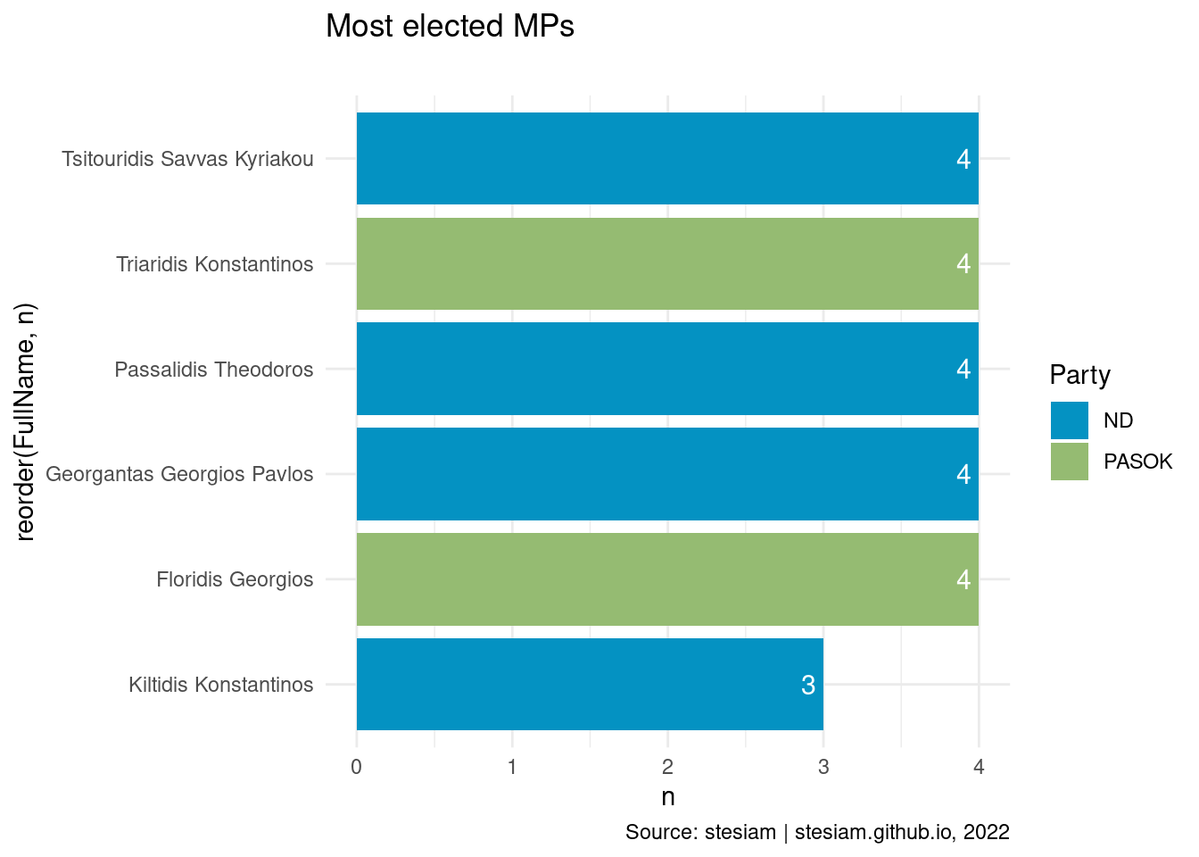
Show the code
constituency_freqs("Kilkis",3)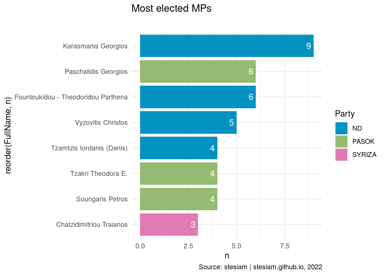
Show the code
constituency_freqs("Pella",3)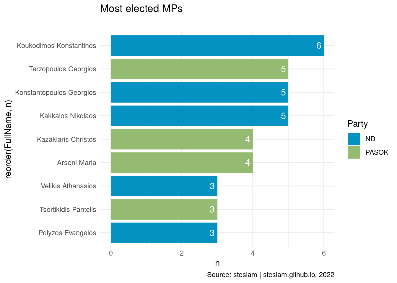
Show the code
constituency_freqs("Pieria",3)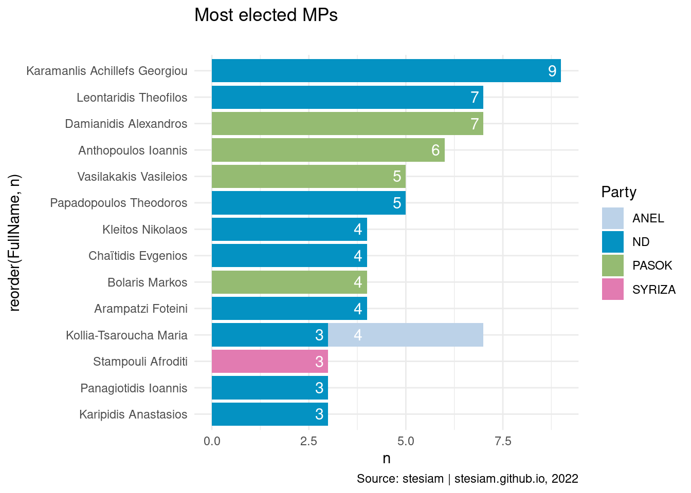
Show the code
constituency_freqs("Serres",3)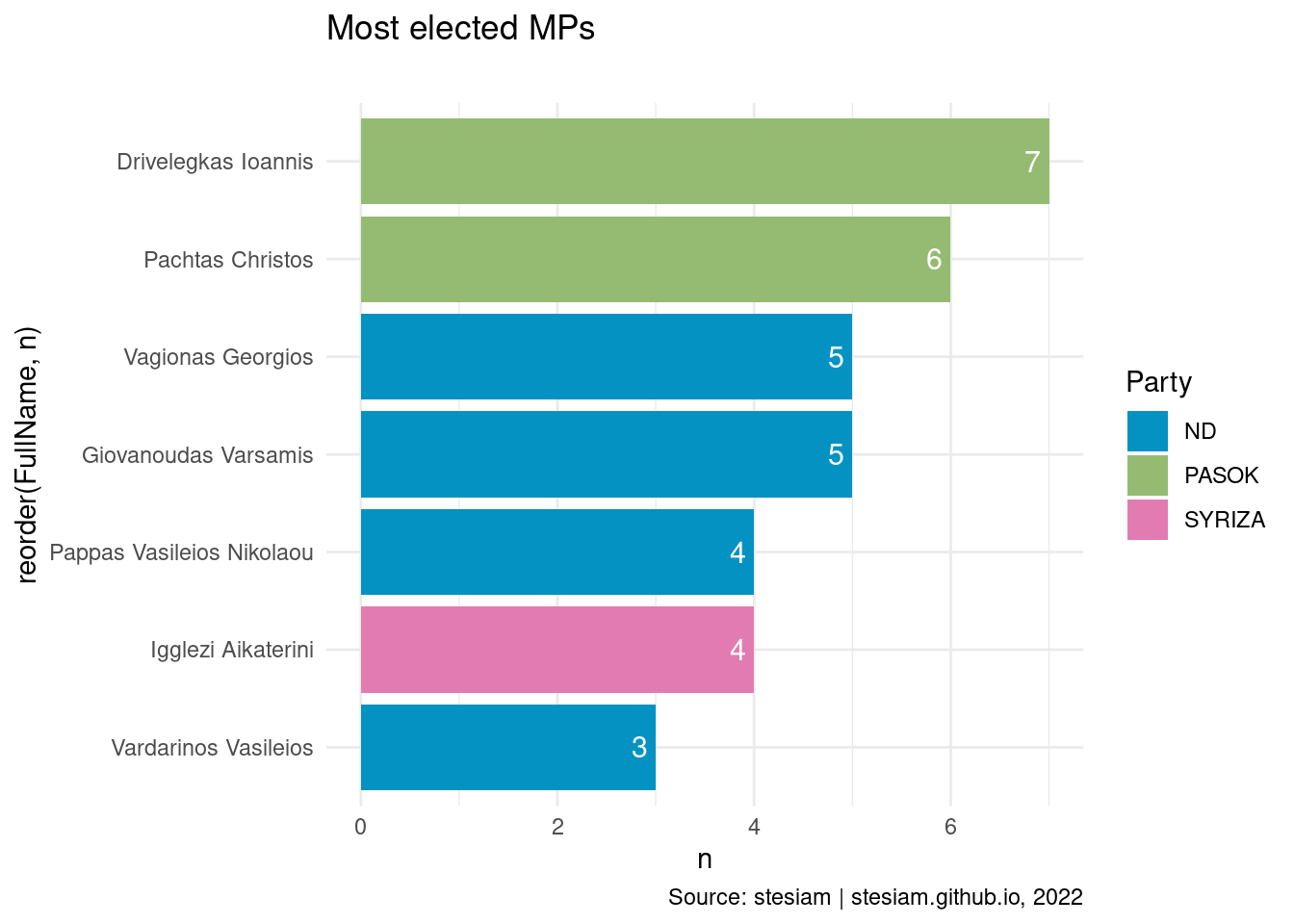
Show the code
constituency_freqs("Halkidiki",3)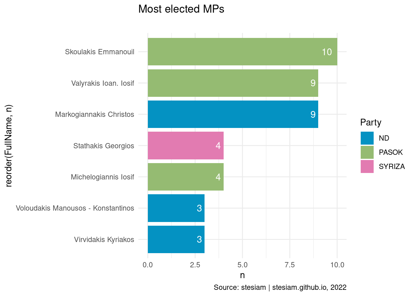
Crete
Show the code
constituency_freqs("Chania",3)
Show the code
#constituency_freqs("Irakleio",3)Show the code
constituency_freqs("Lasithi",3)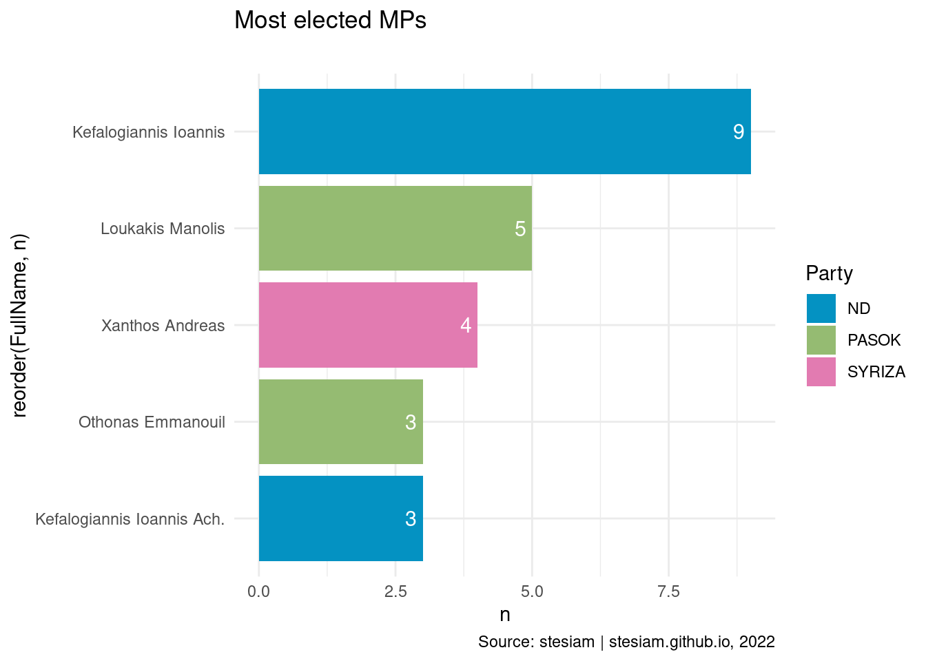
Show the code
constituency_freqs("Rethymno",3)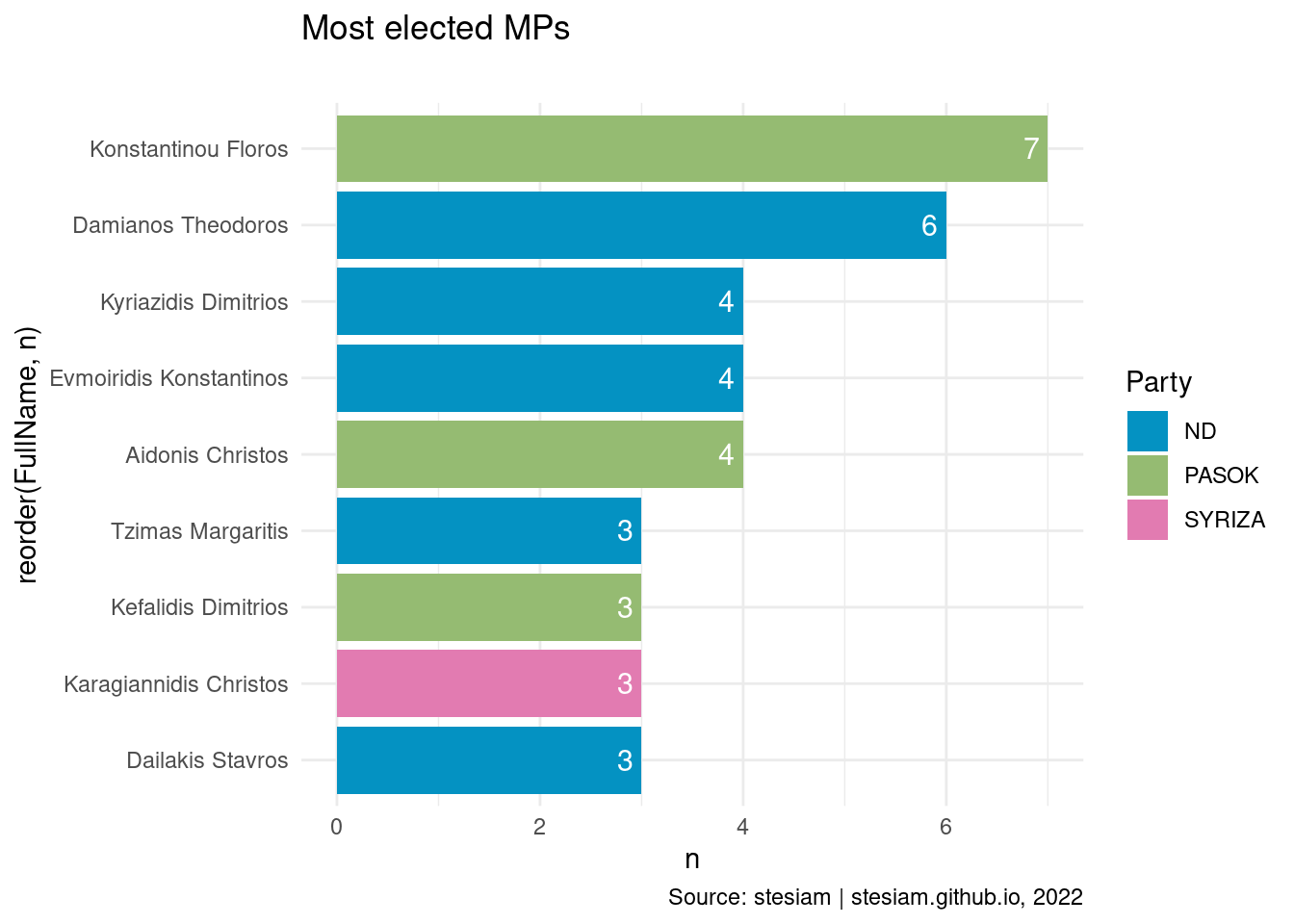
Eastern Macedonia and Thrace
Show the code
constituency_freqs("Drama",3)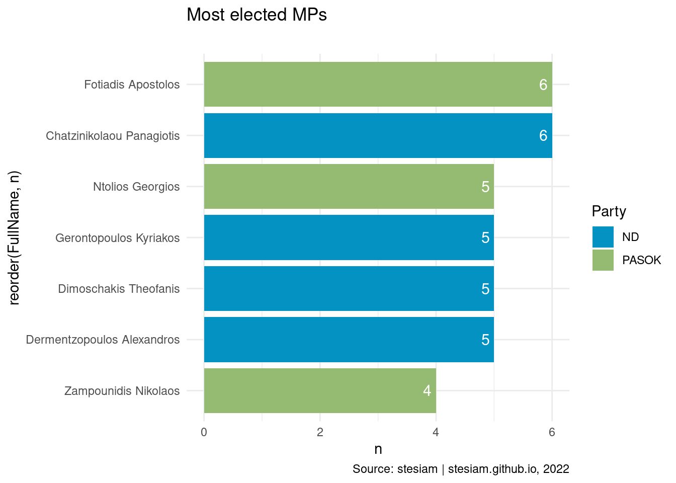
Show the code
constituency_freqs("Evros",4)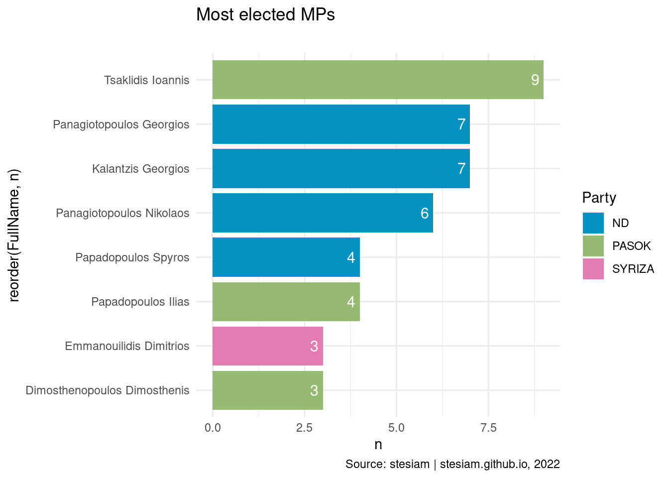
Show the code
constituency_freqs("Kavala",3)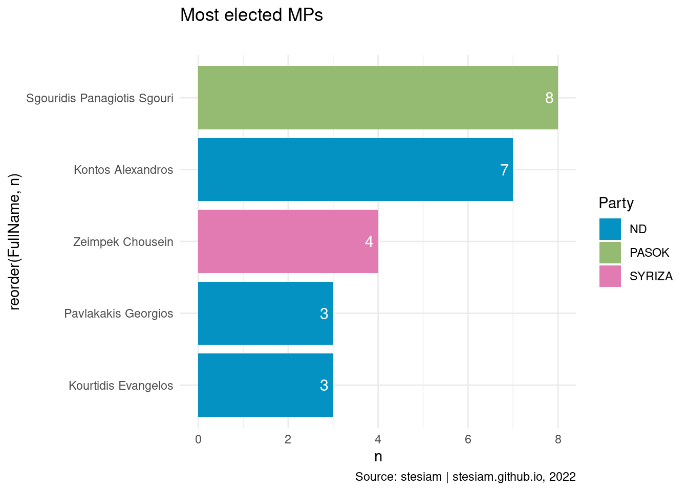
Show the code
constituency_freqs("Xanthi",3)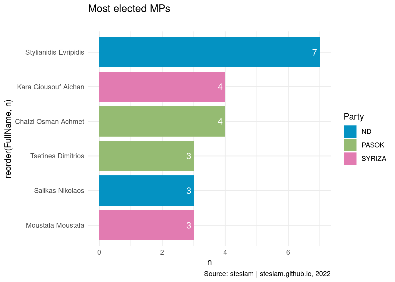
Show the code
constituency_freqs("Rodopi",3)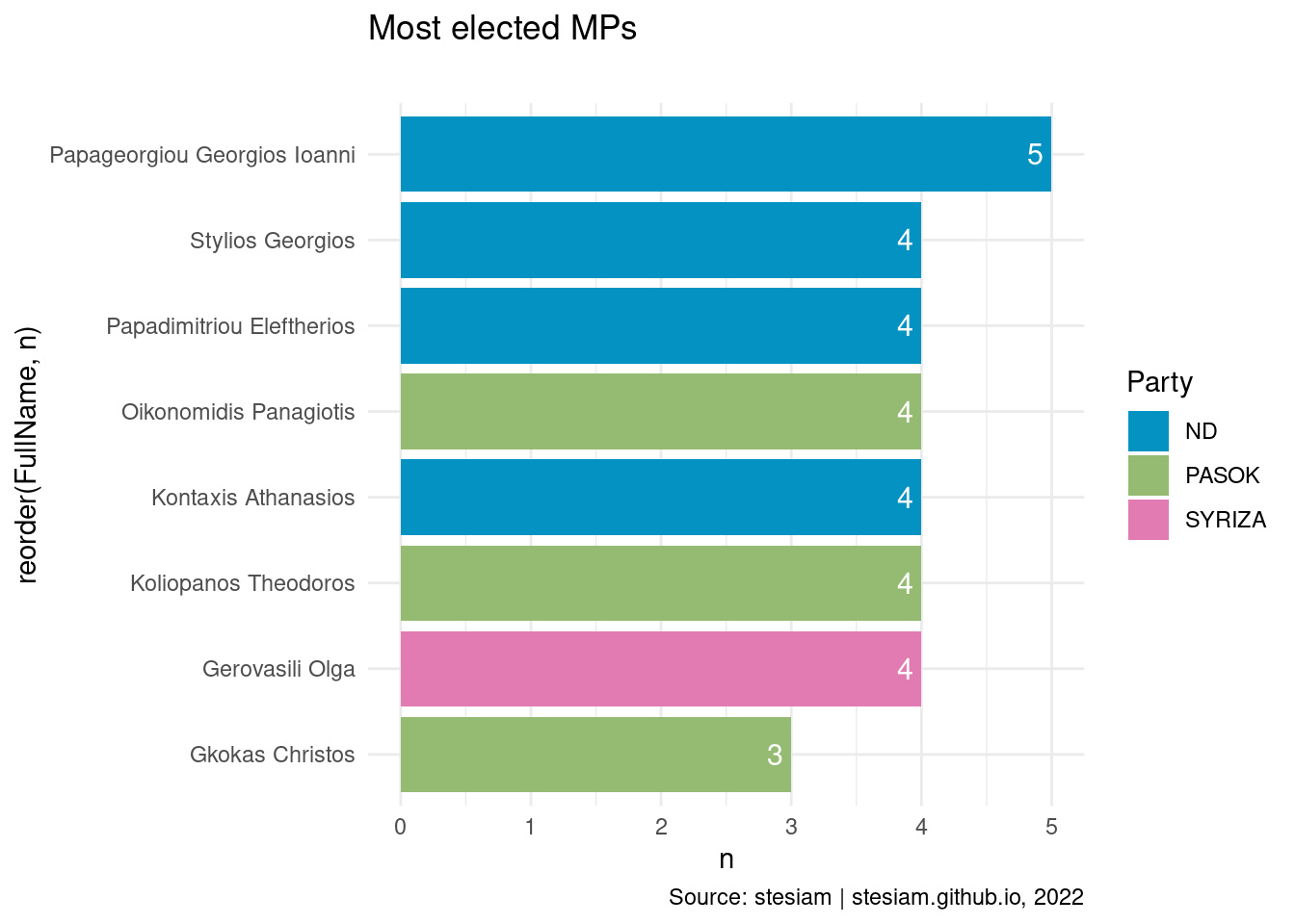
Epirus
Show the code
constituency_freqs("Arta",3)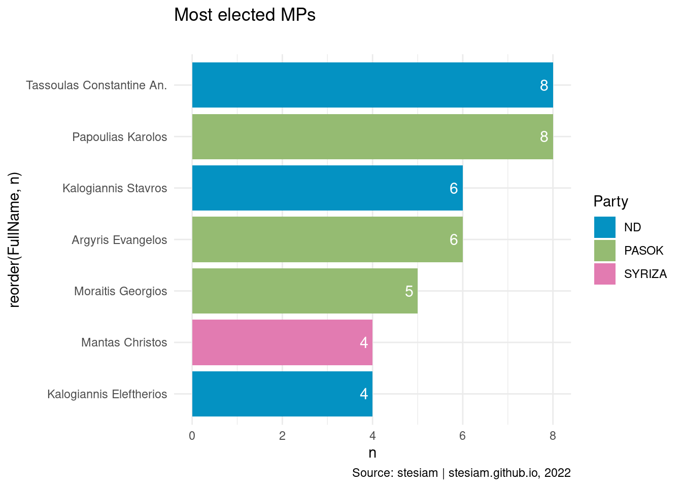
Show the code
constituency_freqs("Ioannina",4)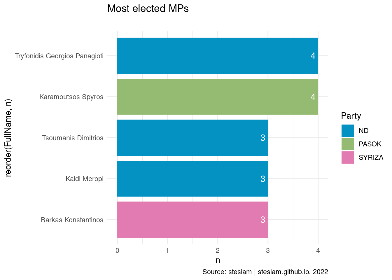
Show the code
constituency_freqs("Preveza",3)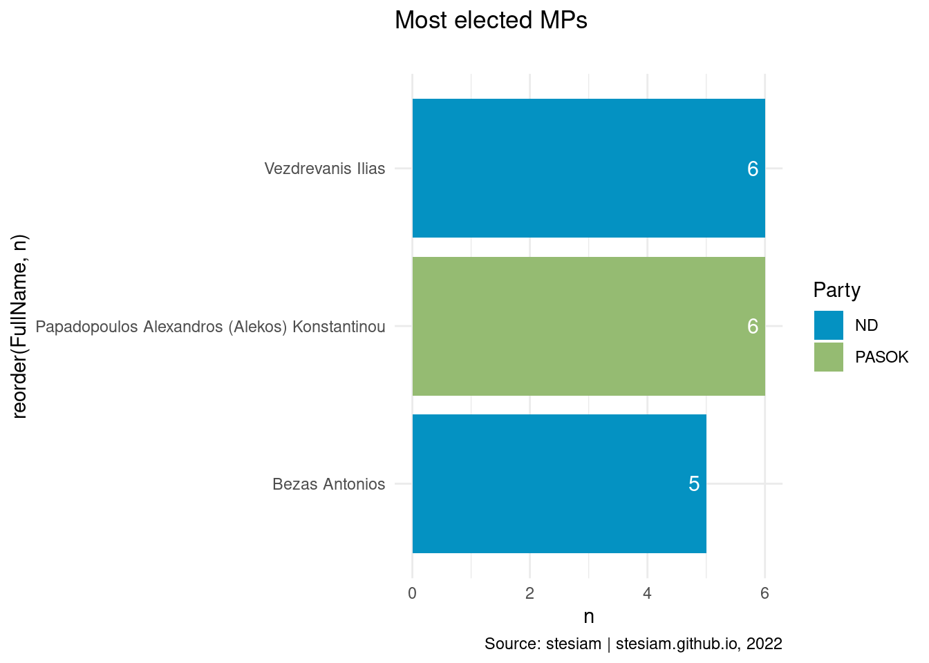
Show the code
constituency_freqs("Thesprotia",3)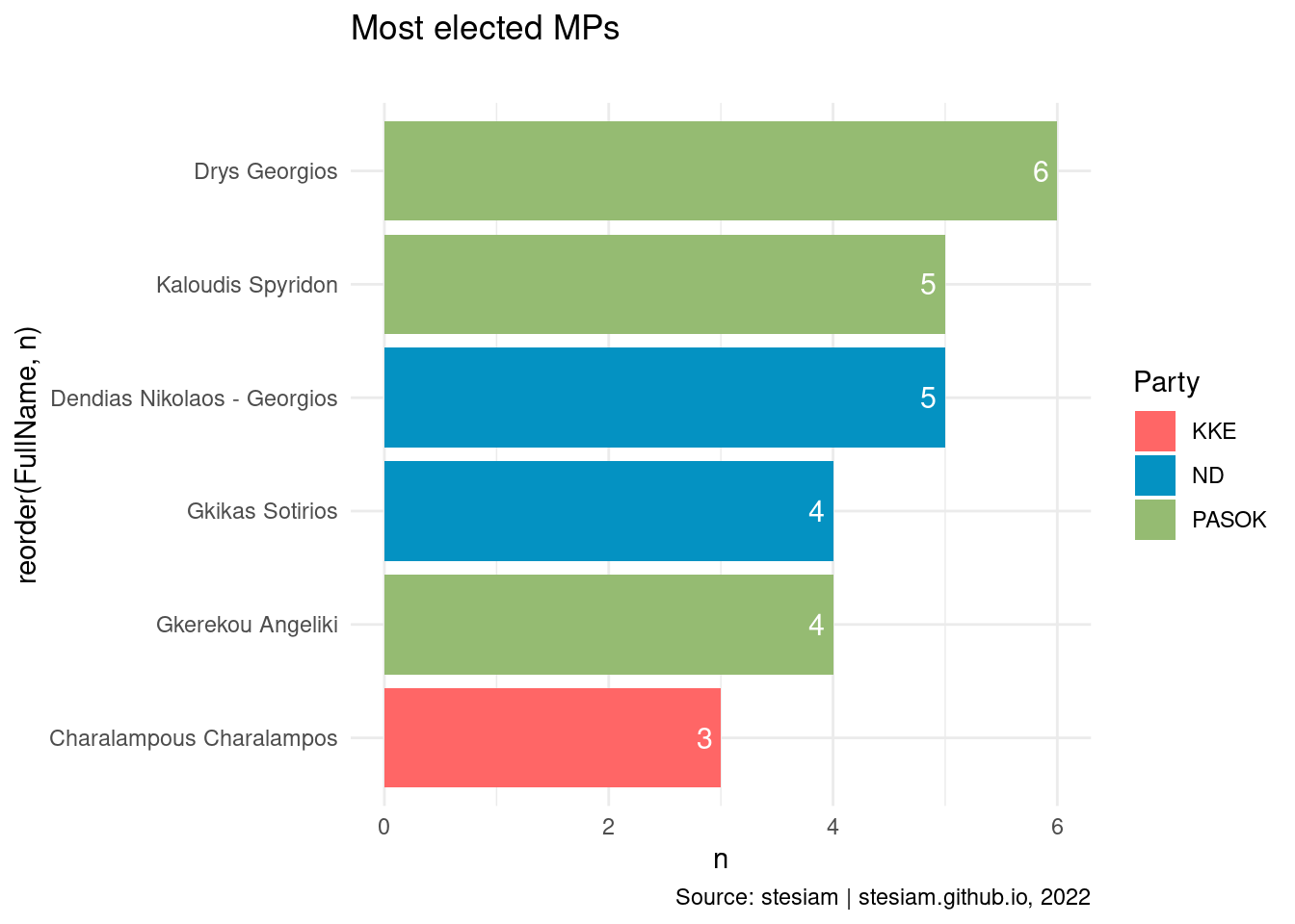
Ionian Islands
Show the code
constituency_freqs("Corfu",3)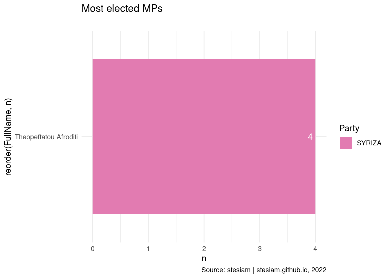
Show the code
constituency_freqs("Kefallonia",3)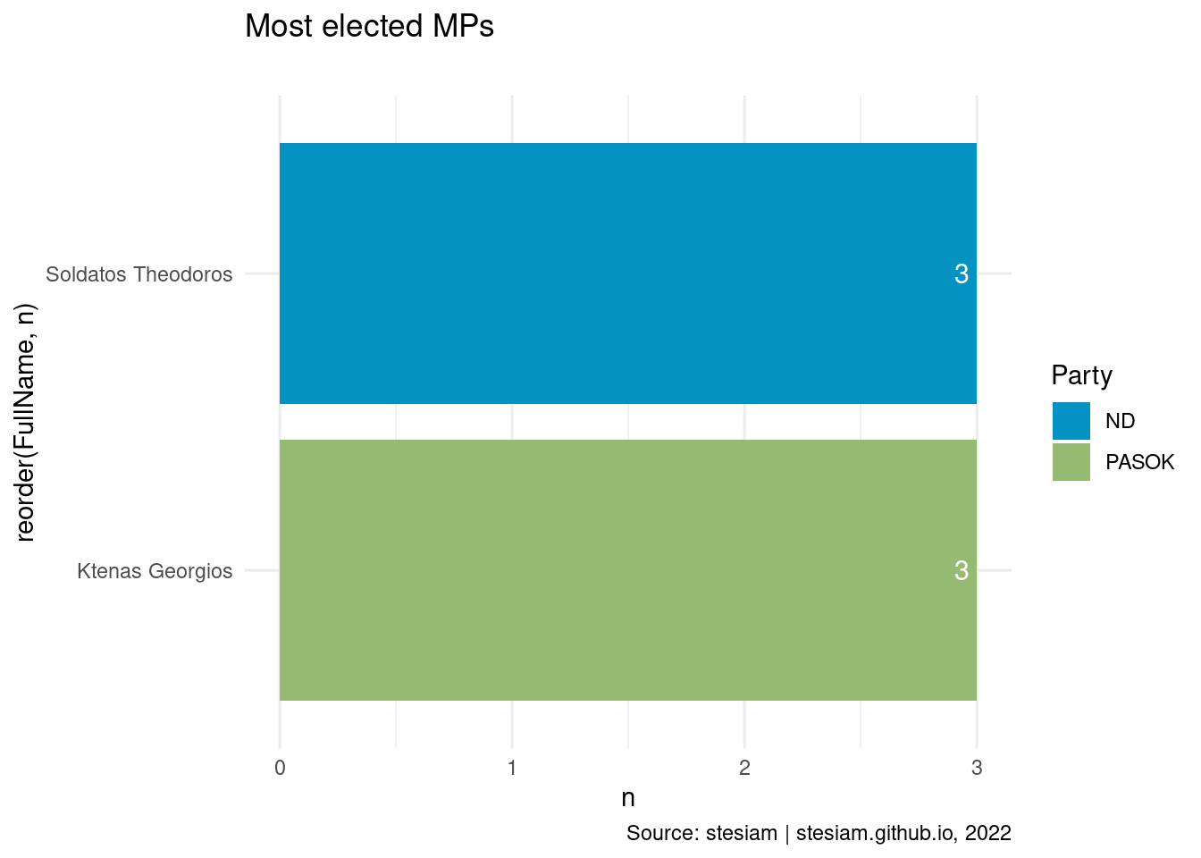
Show the code
constituency_freqs("Lefkada",3)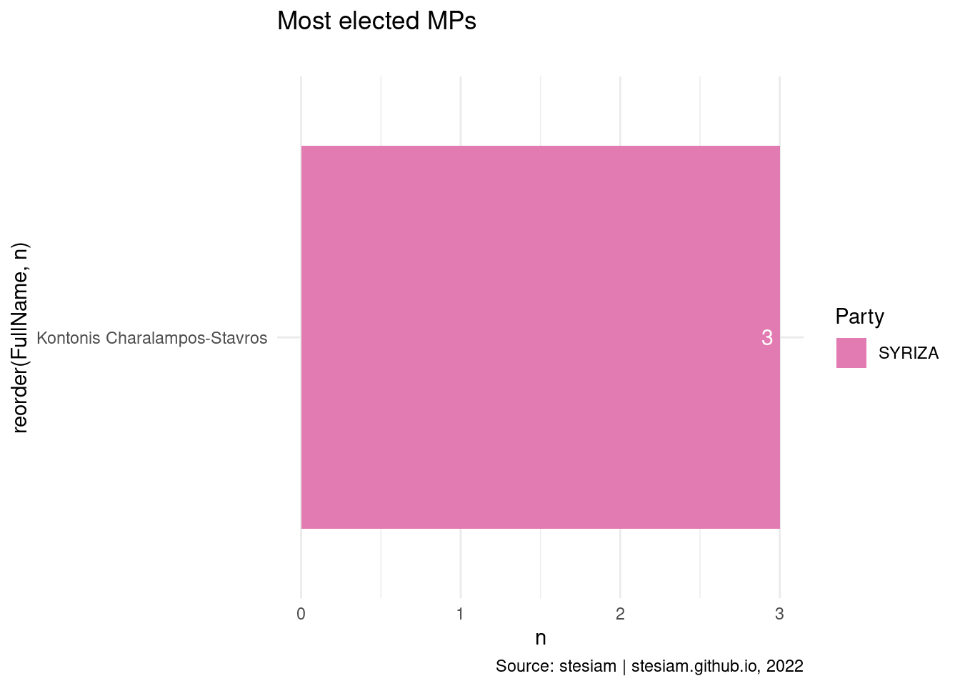
Show the code
constituency_freqs("Zakynthos",3)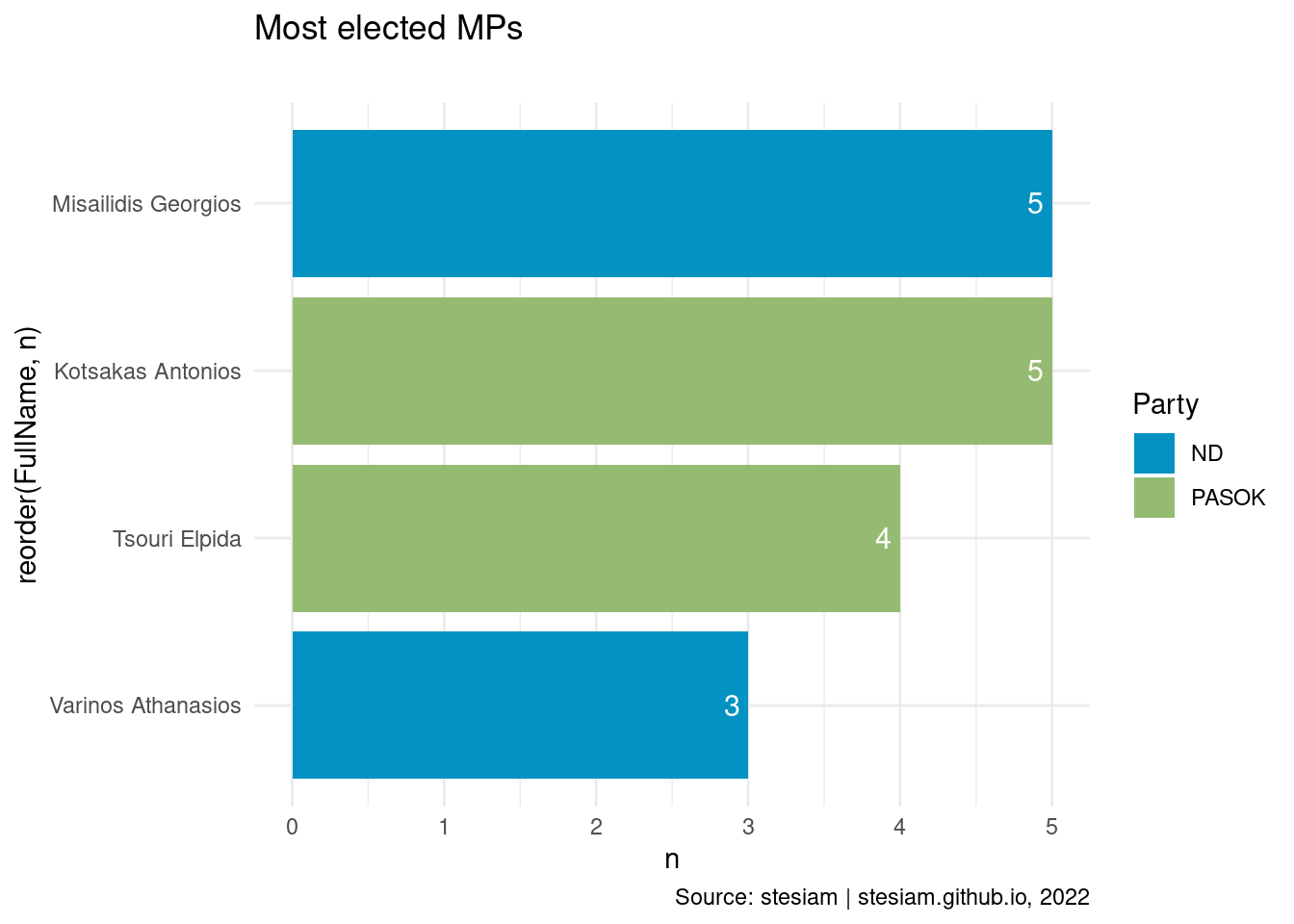
North Aegean
Show the code
constituency_freqs("Chios",3)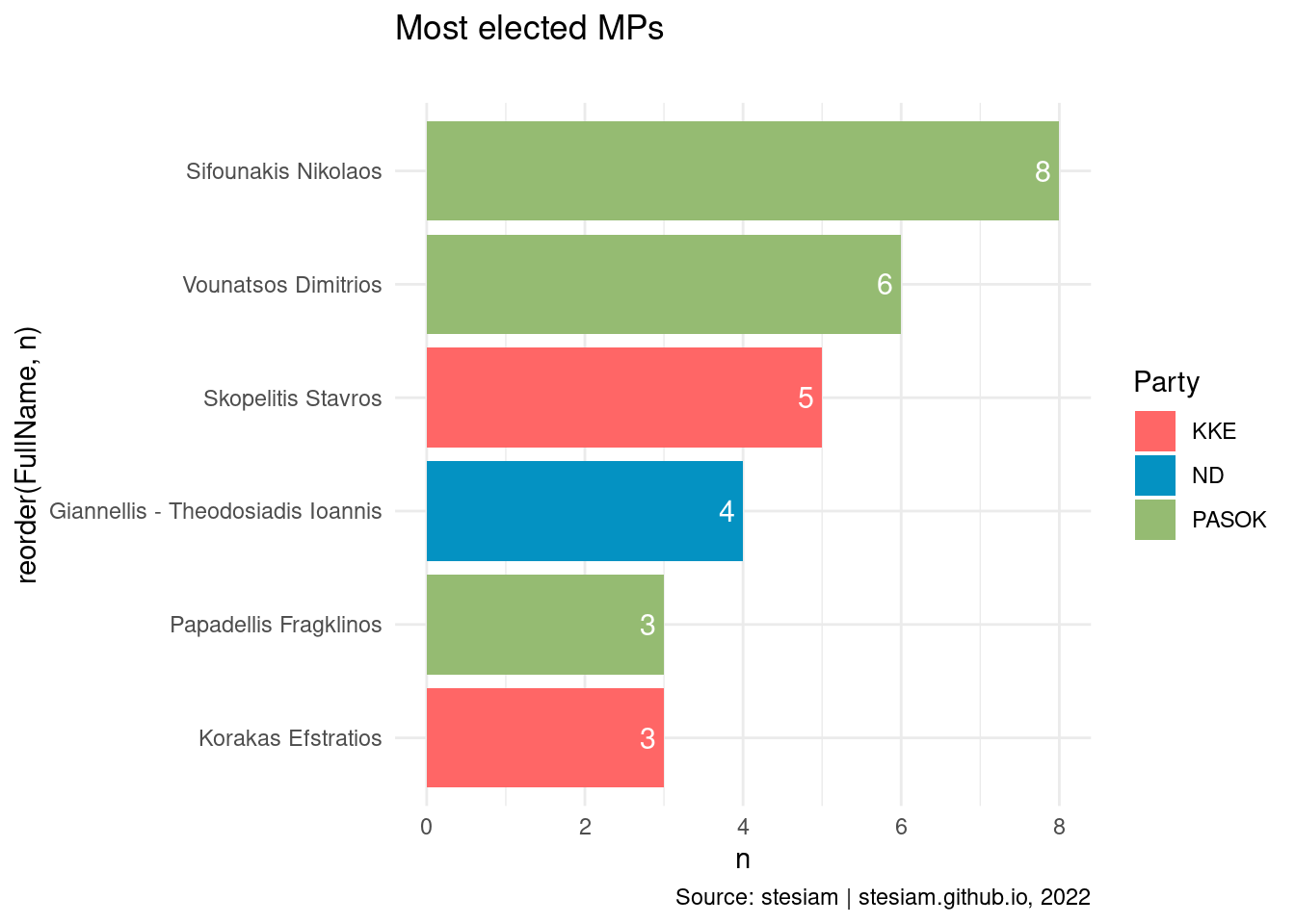
Show the code
constituency_freqs("Lesvos",3)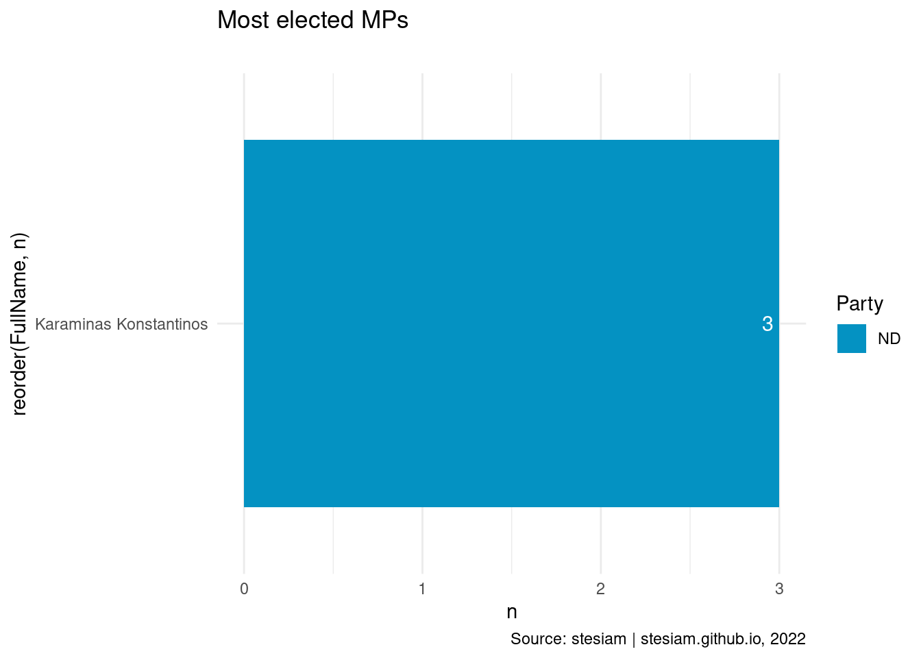
Show the code
constituency_freqs("Samos",3)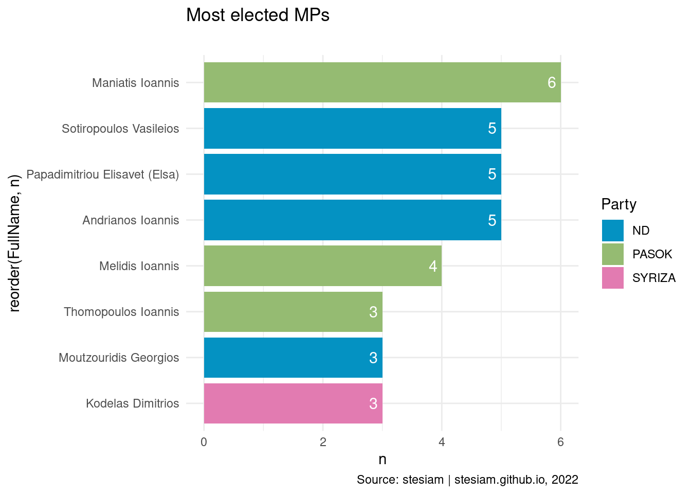
Peloponnese
Show the code
constituency_freqs("Argolida",3)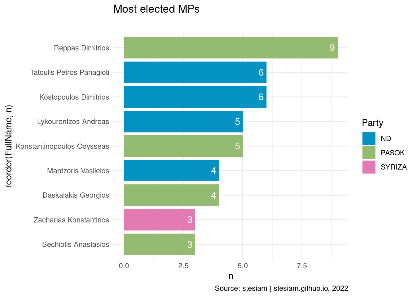
Show the code
constituency_freqs("Arcadia",3)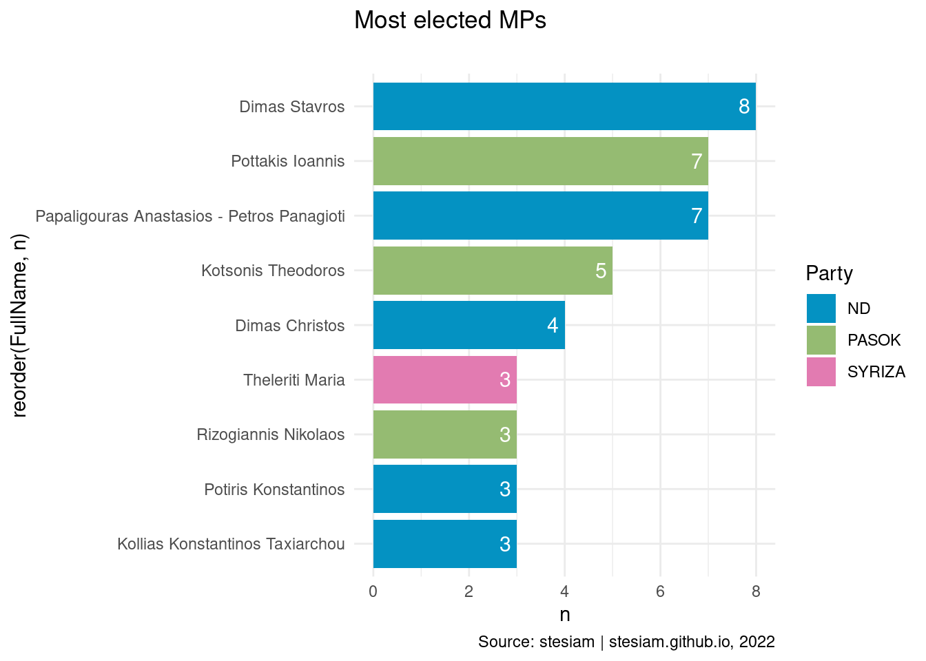
Show the code
constituency_freqs("Korinthia",3)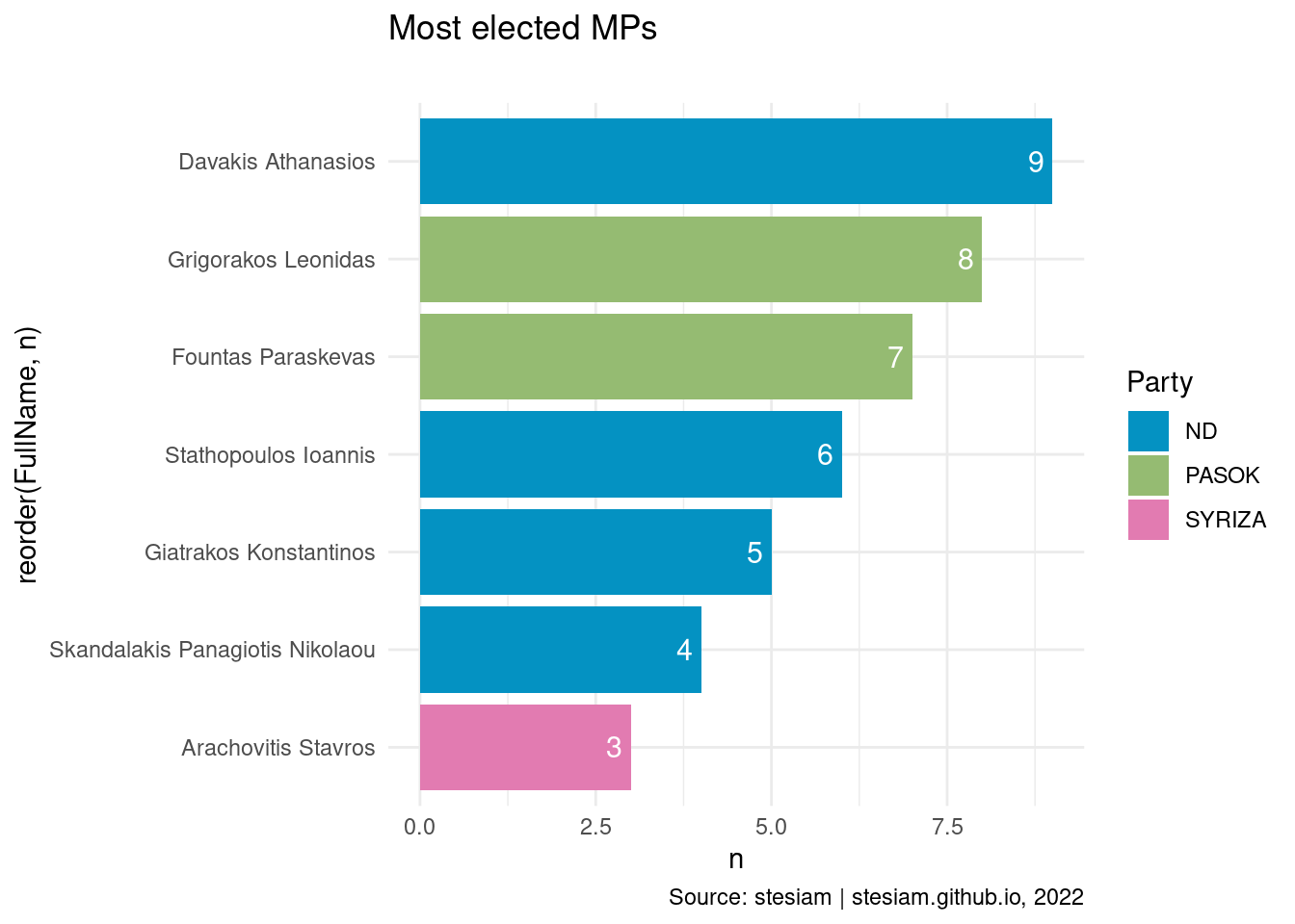
Show the code
constituency_freqs("Lakonia",3)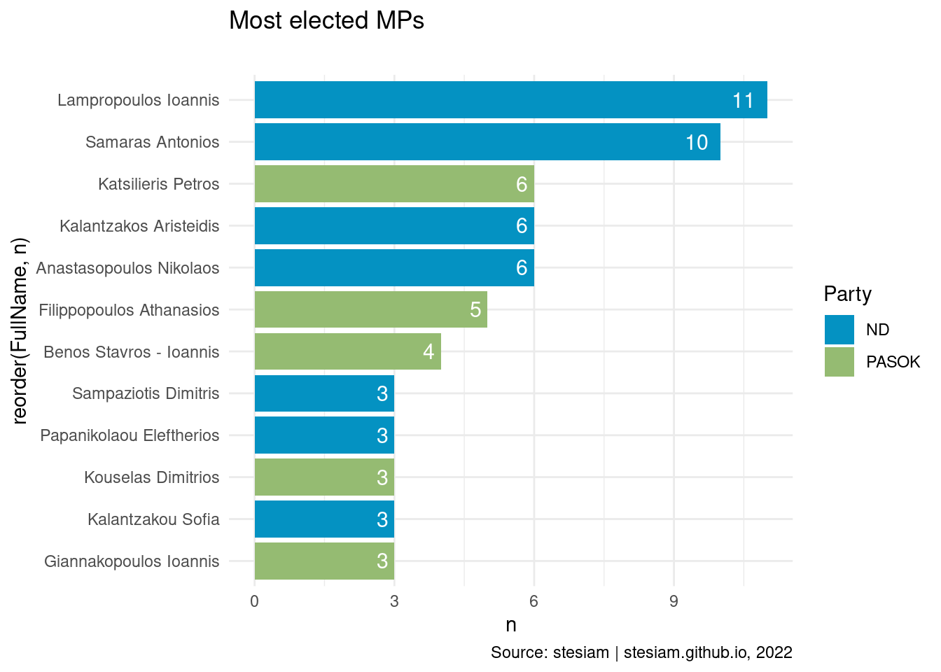
Show the code
constituency_freqs("Messinia",3)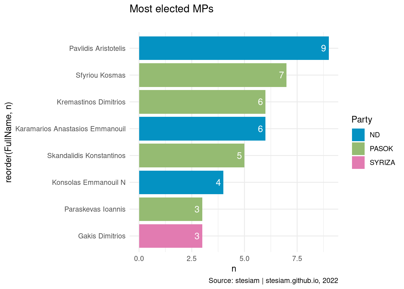
South Aegean
Show the code
constituency_freqs("Dodecanese Islands",3)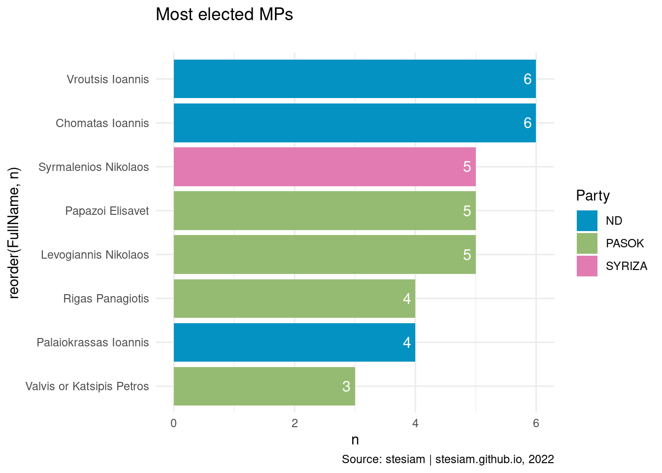
Show the code
constituency_freqs("Cyclades",3)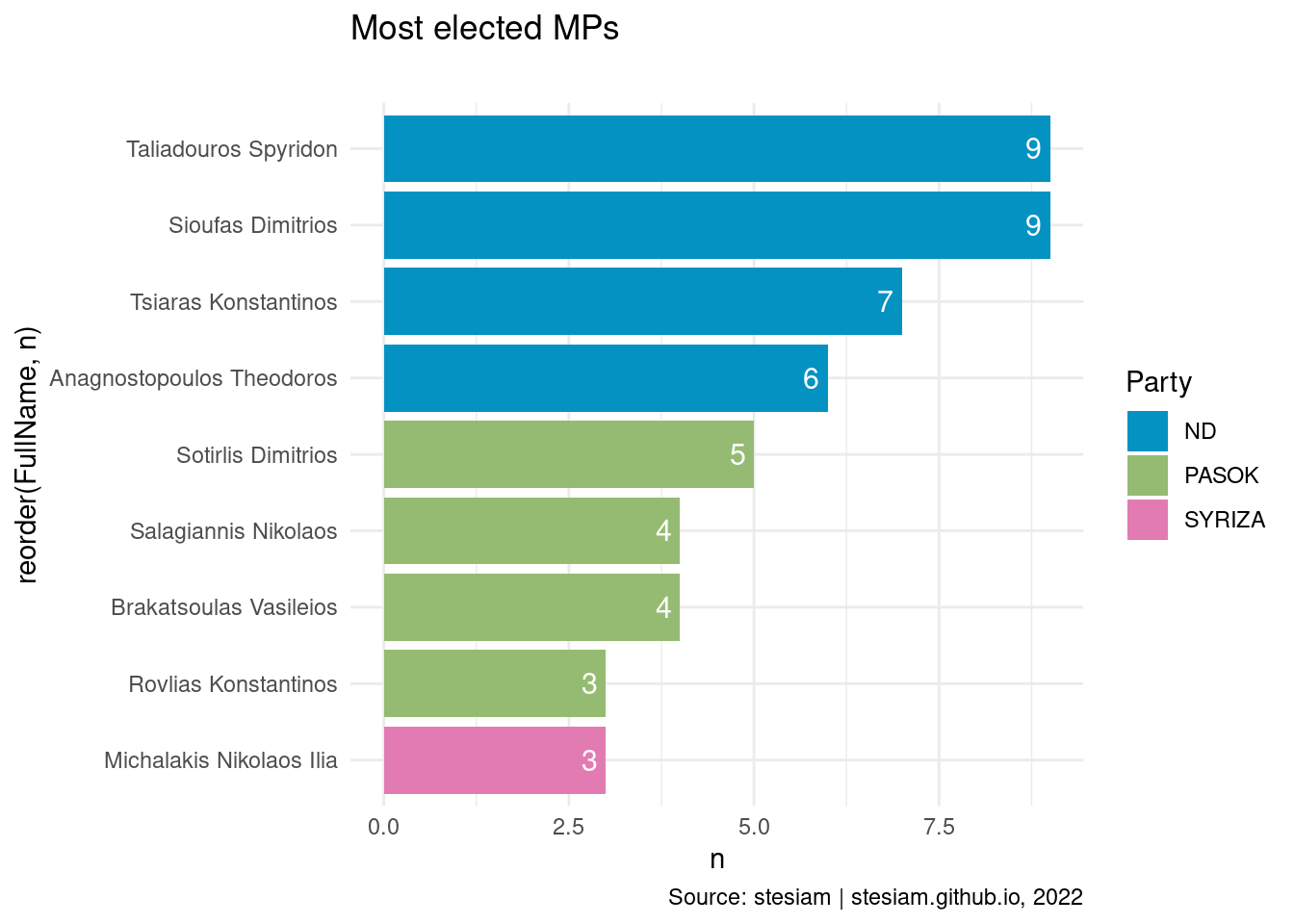
Thessaly
Show the code
constituency_freqs("Karditsa",3)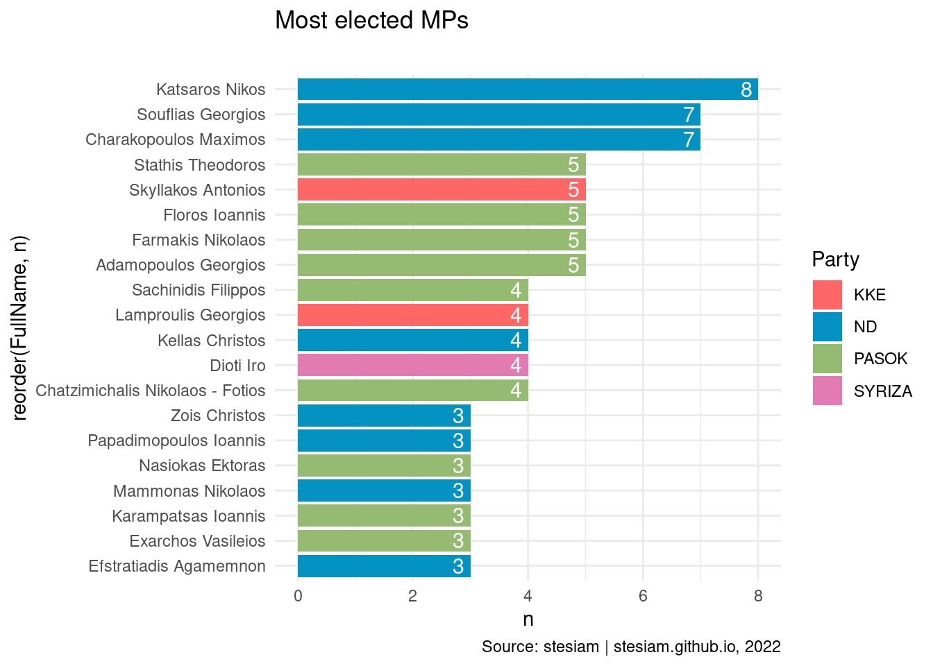
Show the code
constituency_freqs("Larissa",3)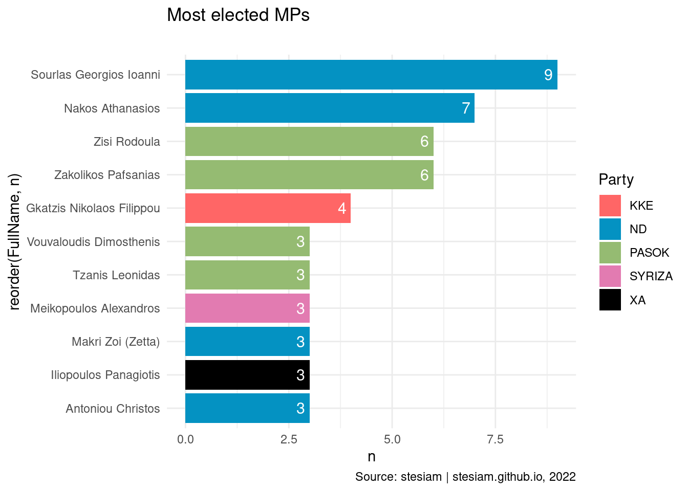
Show the code
constituency_freqs("Magnesia",3)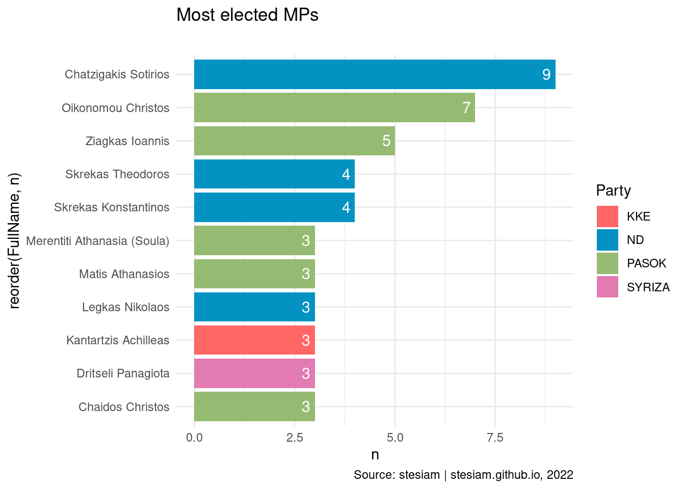
Show the code
constituency_freqs("Trikala",3)
Western Greece
Show the code
constituency_freqs("Achaia",3)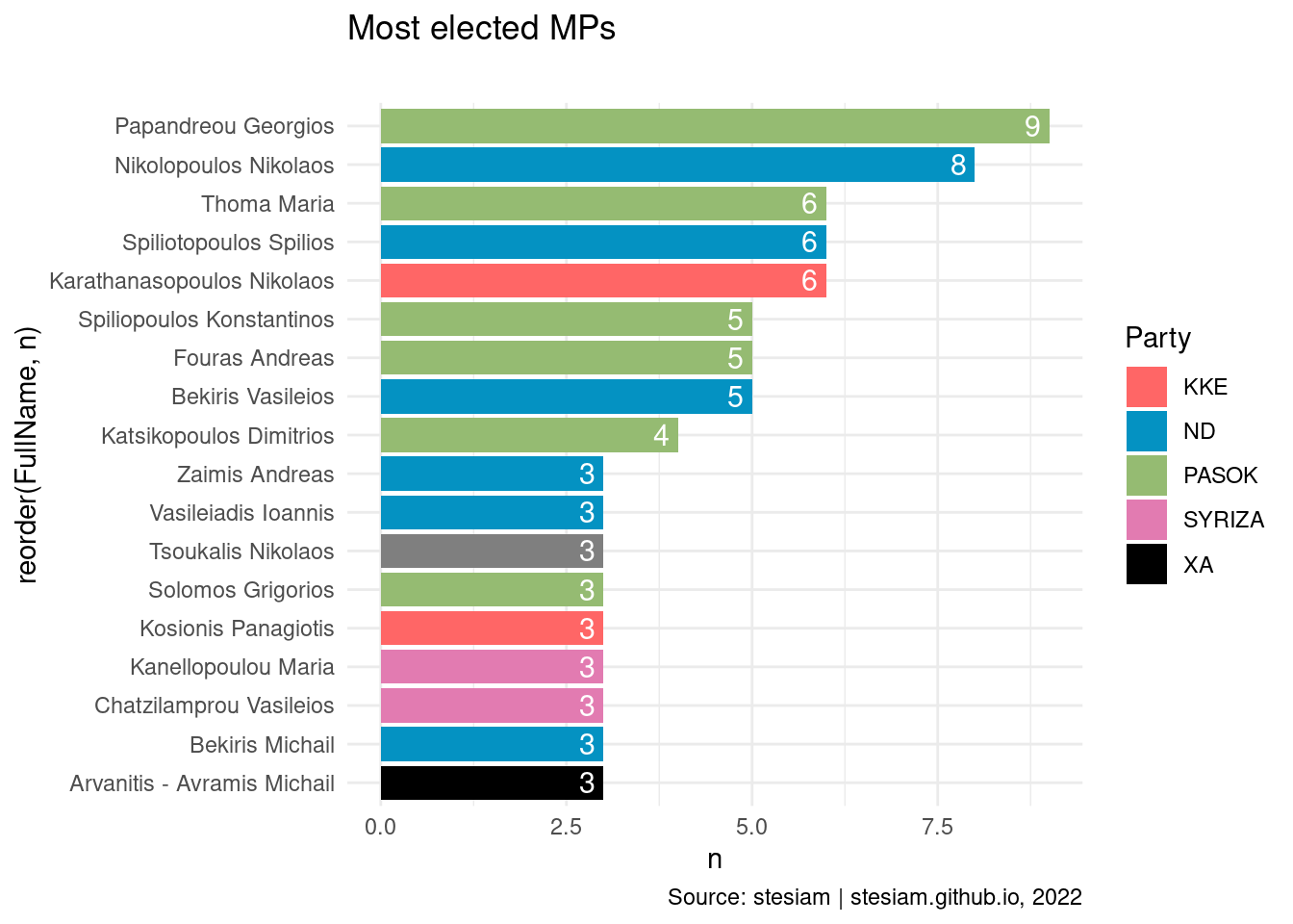
Show the code
#constituency_freqs("Aitoloakarnania",3)Show the code
constituency_freqs("Ileia",3)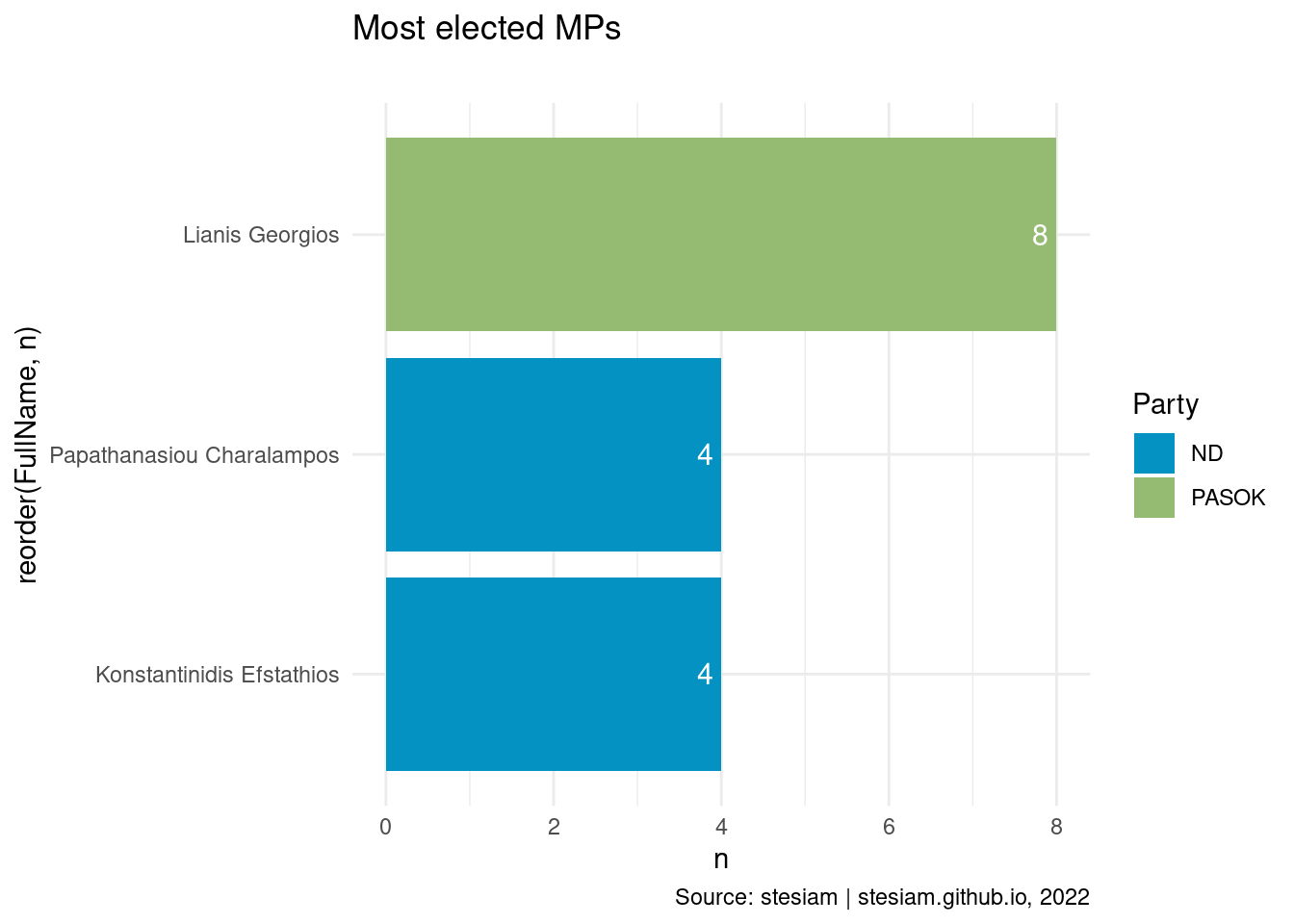
Western Macedonia
Show the code
constituency_freqs("Florina",3)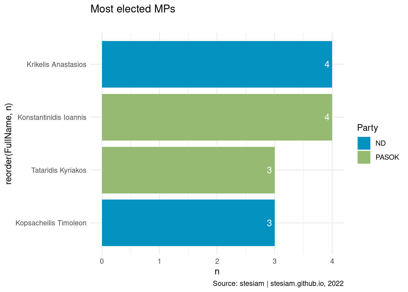
Show the code
constituency_freqs("Grevena",3)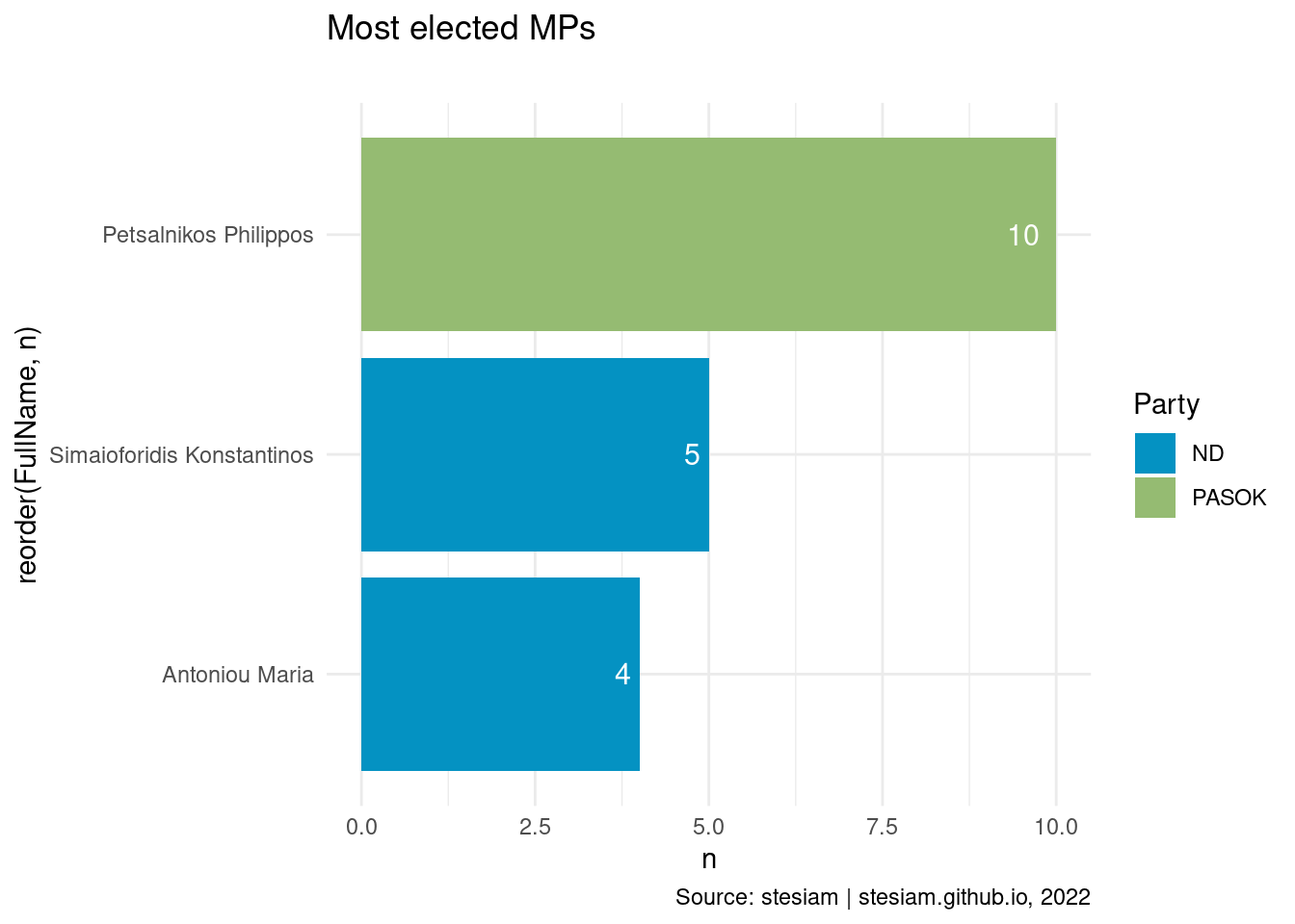
Show the code
constituency_freqs("Kastoria",3)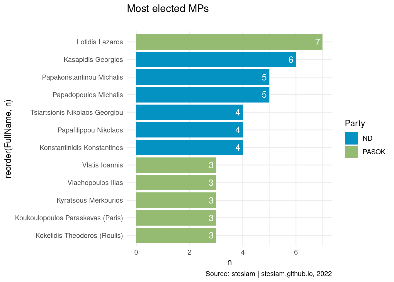
Show the code
constituency_freqs("Kozani",3)
Acknowledgments
Image by Leonhard Niederwimmer from Pixabay
Data are from mine repository on GitHub. Original data are from Hellenic’s Parliament website
References
Citation
@online{2022,
  author = {, stesiam},
  title = {EDA on {Greek} {Parliament}},
  date = {2022-10-10},
  url = {https://stesiam.com/posts/eda-greek-parliament/},
  langid = {en}
}